Chapter 3 Blocking
The completely randomised design (CRD) works well when there is sufficient homogeneous experimental units to perform the whole experiment under the same, or very similar, conditions and there are no restrictions on the randomisation of treatments to units. The only systematic (non-random) differences in the observed responses result from differences between the treatments. While such designs are commonly and successfully used, especially in smaller experiments, their application can often be unrealistic or impractical in many settings.
A common way in which the CRD fails is a lack of sufficiently similar experimental units. If there are systemtic differences between different batches, or blocks of units, these differences should be taken into account in both the allocation of treatments to units and the modelling of the resultant data. Otherwise, block-to-block differences may bias treatment comparisons and/or inflate our estimate of the background variability and hence reduce our ability to detect important treatment effects.
Example 3.1 Steel bar experiment (Morris, 2011, ch. 4)
Kocaoz et al. (2005) described an experiment to assess the strength of steel reinforcement bars from \(t=4\) coatings18 (treatments). In total \(n=32\) different bars (units) were available, but the testing process meant sets of four bars were tested together. To account for potential test-specific features (e.g. environmental or operational), these different test sets were assumed to form \(b=8\) blocks of size \(k=4\). The data are shown in Table 3.1 below.
bar <- data.frame(coating = rep(factor(1:4), 8),
                   block = rep(factor(1:8), rep(4, 8)),
                   strength = c(136, 147, 138, 149, 136, 143, 122, 153, 150, 142, 131, 136,
                                   155, 148, 130, 129, 145, 149, 136, 139, 150, 149, 147, 144,
                                   147, 150, 125, 140, 148, 149, 118, 145)
                     )
knitr::kable(
 tidyr::pivot_wider(bar, names_from = coating, values_from = strength),
 col.names = c("Block", paste("Coating", 1:4)),
 caption = "Steel bar experiment: tensile strength values (kliograms per square inch, ksi) from steel bars with four different coatings."
)| Block | Coating 1 | Coating 2 | Coating 3 | Coating 4 |
|---|---|---|---|---|
| 1 | 136 | 147 | 138 | 149 |
| 2 | 136 | 143 | 122 | 153 |
| 3 | 150 | 142 | 131 | 136 |
| 4 | 155 | 148 | 130 | 129 |
| 5 | 145 | 149 | 136 | 139 |
| 6 | 150 | 149 | 147 | 144 |
| 7 | 147 | 150 | 125 | 140 |
| 8 | 148 | 149 | 118 | 145 |
Here, each block has size 4, which is equal to the number of treatments in the experiment, and each treatment is applied in each block. This is an example of a randomised complete block design.
We can study the data graphically, plotting by treatment and by block.
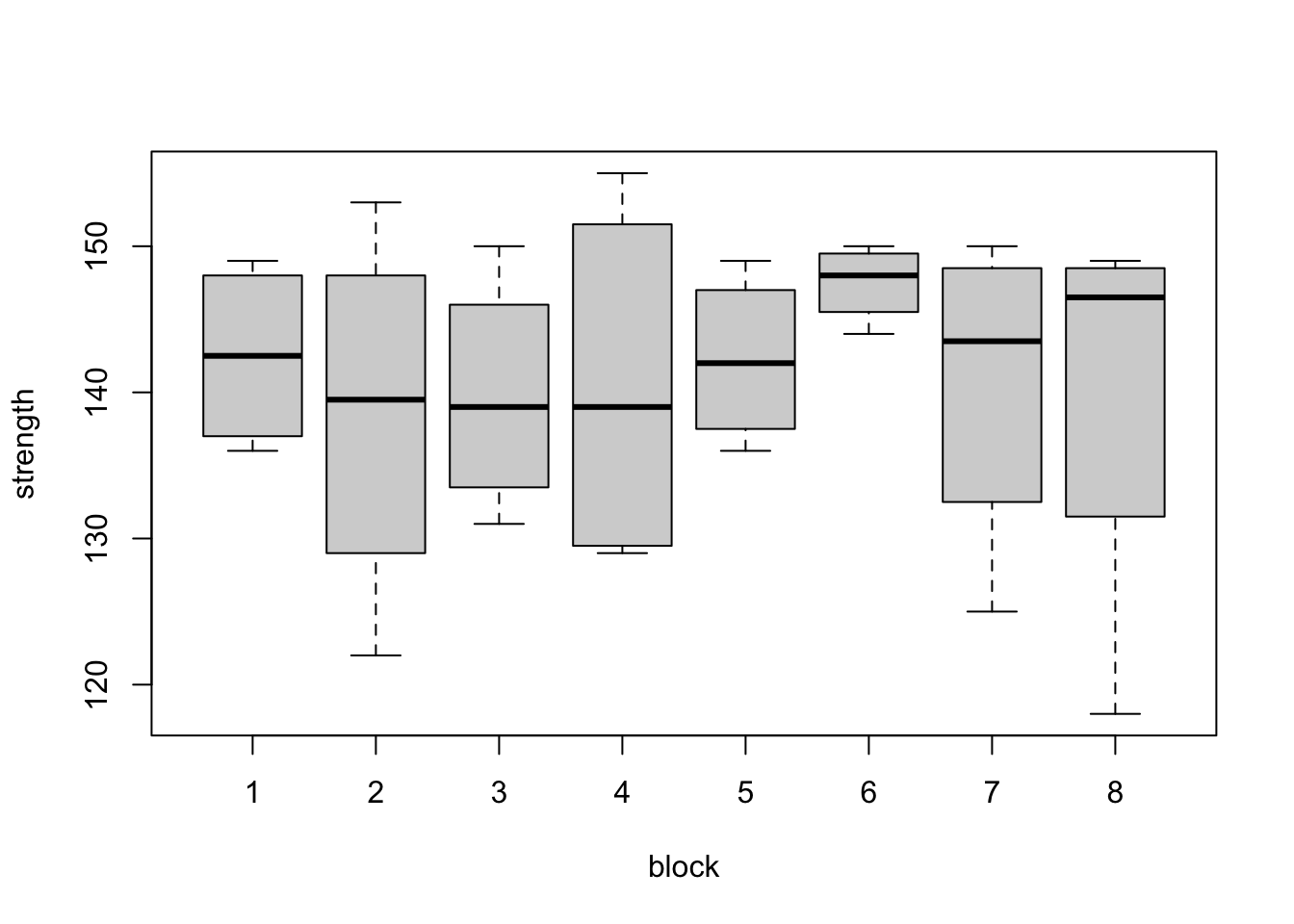
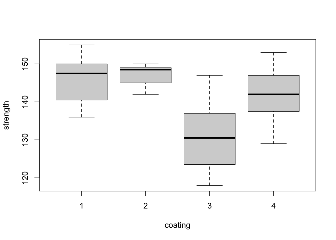
Figure 3.1: Steel bar experiment: distributions of tensile strength (ksi) from the eight blocks (top) and the four coatings (bottom).
The box plots within each plot in Figure 3.1 are comparable, as every treatment has occured with every block the same number of times (once). For example, when we compare the box plots for treatments 1 and 3, we know each of then display one observation from each block. Therefore, differences between treatments will not be influenced by large differences between blocks. This balance makes our analysis more straighforward. By eye, it appears here there may be differences between coating 3 and the other three coatings.
Example 3.2 Tyre experiment (Wu and Hamada, 2009, ch. 3)
Davies (1954), p.200, examined the effect of \(t=4\) different rubber compounds (treatments) on the lifetime of a tyre. Each tyre is only large enough to split into \(k=3\) segments whilst still containing a representative amount of each compound. When tested, each tyre is subjected to the same road conditions, and hence is treated as a block. A design with \(b=4\) blocks was used, as displayed in Table 3.2.
tyre <- data.frame(compound = as.factor(c(1, 2, 3, 1, 2, 4, 1, 3, 4, 2, 3, 4)),
                   block = rep(factor(1:4), rep(3, 4)),
                   wear = c(238, 238, 279, 196, 213, 308, 254, 334, 367, 312, 421, 412)
                     )
options(knitr.kable.NA = '')
knitr::kable(
 tidyr::pivot_wider(tyre, names_from = compound, values_from = wear),
 col.names = c("Block", paste("Compound", 1:4)),
 caption = "Tyre experiment: relative wear measurements (unitless) from tires made with four different rubber compounds."
)| Block | Compound 1 | Compound 2 | Compound 3 | Compound 4 |
|---|---|---|---|---|
| 1 | 238 | 238 | 279 | |
| 2 | 196 | 213 | 308 | |
| 3 | 254 | 334 | 367 | |
| 4 | 312 | 421 | 412 |
Here, each block has size \(k=3\), which is smaller than the number of treatments (\(t=4\)). Hence, each block cannot contain an application of each treatment. This is an example of an incomplete block design.
Graphical exploration of the data is a little more problematic in this example. As each treatment does not occur in each block, box plots such as Figure 3.2 are not as informative. Do compounds three and four have higher average wear because they were the only compounds to both occur in blocks 3 and 4? Or do blocks 3 and 4 have a higher mean because they contain both compounds 3 and 4? The design cannot help us entirely disentangle the impact of blocks and treatments19. In our modelling, we will assume variation should first be described by blocks (which are generally fixed aspects of the experiment) and then treatments (which are more directly under the experimenter’s control).
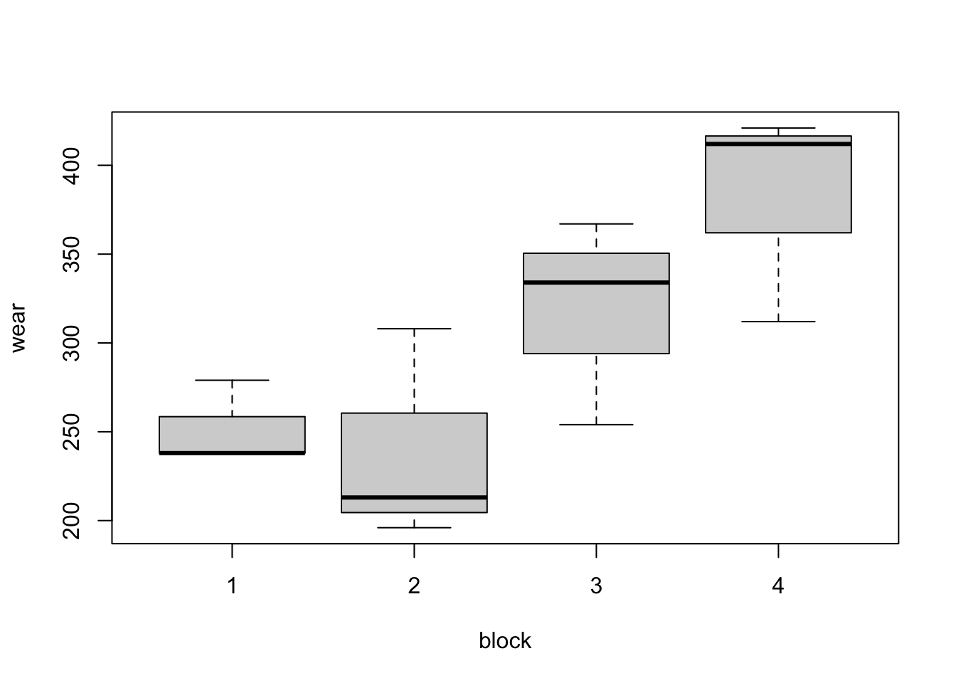
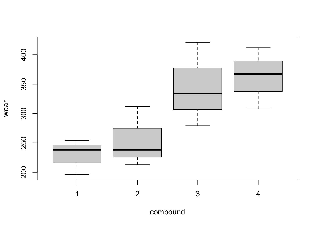
Figure 3.2: Tyre experiment: distributions of wear from the four blocks (top) and the four compounds (bottom).
3.1 Unit-block-treatment model
If \(n_{ij}\) is the number of times treatment \(j\) occurs in block \(i\), a common statistical model to describe data from a blocked experiment has the form
\[\begin{equation} y_{ijl} = \mu + \beta_i + \tau_j + \varepsilon_{ijl}\,, \qquad i = 1,\ldots, b; j = 1, \ldots, t; l = 1,\ldots,n_{ij}\,, \tag{3.1} \end{equation}\] where \(y_{ijl}\) is the response from the \(l\)th application of the \(j\)th treatment in the \(i\)th block, \(\mu\) is a constant parameter, \(\beta_i\) is the effect of the \(i\)th block, \(\tau_j\) is the effect of treatment \(j\), and \(\varepsilon_{ijl}\sim N(0, \sigma^2)\) are once again random individual effects from each experimental unit, assumed independent. The total number of runs in the experiment is given by \(n = \sum_{i=1}^b\sum_{j=1}^t n_{ij}\).
For Example 3.1, there are \(t=4\) experiments, \(b = 8\) blocks and each treatment occurs once in each block, so \(n_{ij} = 1\) for all \(i, j\). In Example 3.2, there are again \(t=4\) treatments but now only \(b=4\) blocks and not every treatment occurs in every block. In fact, we have \(n_{11} = n_{12} = n_{13} = 1\), \(n_{14} = 0\), \(n_{21} = n_{22} =n_{24} = 1\), \(n_{23} = 0\), \(n_{31} = n_{33} =n_{34} = 1\), \(n_{32} = 0\), \(n_{41} = 0\) and \(n_{42} = n_{43} =n_{44} = 1\).
Writing model (3.1) is matrix form as a partitioned linear model, we obtain
\[\begin{equation} \boldsymbol{y}= \mu\boldsymbol{1}_n + X_1\boldsymbol{\beta} + X_2\boldsymbol{\tau} + \boldsymbol{\varepsilon}\,, \tag{3.2} \end{equation}\]
with \(\boldsymbol{y}\) the \(n\)-vector of responses, \(X_1\) and \(X_2\) \(n\times b\) and \(n\times t\) model matrices for blocks and treatments, respectively, \(\boldsymbol{\beta} = (\beta_1,\ldots, \beta_b)^{\mathrm{T}}\), \(\boldsymbol{\tau} = (\tau_1,\ldots, \tau_t)^{\mathrm{T}}\) and \(\boldsymbol{\varepsilon}\) the \(n\)-vector of errors.
In equation(3.2), assuming without loss of generality that runs of the experiment are ordered by block, the matrix \(X_1\) has the form
\[ X_1 = \bigoplus_{i = 1}^b \boldsymbol{1}_{k_i} = \begin{bmatrix} \boldsymbol{1}_{k_1} & \boldsymbol{0}_{k_1} & \cdots & \boldsymbol{0}_{k_1} \\ \boldsymbol{0}_{k_2} & \boldsymbol{1}_{k_2} & \cdots & \boldsymbol{0}_{k_2} \\ \vdots & & \ddots & \vdots \\ \boldsymbol{0}_{k_b} & \boldsymbol{0}_{k_b} & \cdots & \boldsymbol{1}_{k_b} \\ \end{bmatrix}\,, \] where \(k_i = \sum_{j=1}^t n_{ij}\), the number of units in the \(i\)th block. The structure of matrix \(X_2\) is harder to describe so succinctly, but each row includes a single non-zero entry, equal to one, indicating which treatment was applied in that run of the experiment. The first \(k_1\) rows correspond to block 1, the second \(k_2\) to block 2, and so on. We will see special cases later.
3.2 Normal equations
Writing as a partitioned model \(\boldsymbol{y}= W\boldsymbol{\alpha} + \boldsymbol{\varepsilon}\), with \(W = [\boldsymbol{1} | X_1 | X_2]\) and \(\boldsymbol{\alpha}^{\mathrm{T}} = [\mu | \boldsymbol{\beta}^{\mathrm{T}} | \boldsymbol{\tau}^{\mathrm{T}}]\), the least squares normal equations
\[\begin{equation} W^{\mathrm{T}}W \hat{\boldsymbol{\alpha}} = W^{\mathrm{T}}\boldsymbol{y} \tag{3.3} \end{equation}\]
can be written as a set of three matrix equations:
\[\begin{align} n\hat{\mu} + \boldsymbol{1}_n^{\mathrm{T}}X_1\hat{\boldsymbol{\beta}} + \boldsymbol{1}_n^{\mathrm{T}}X_2\hat{\boldsymbol{\tau}} & = \boldsymbol{1}_n^{\mathrm{T}}\boldsymbol{y}\,, \tag{3.4}\\ X_1^{\mathrm{T}}\boldsymbol{1}_n\hat{\mu} + X_1^{\mathrm{T}}X_1\hat{\boldsymbol{\beta}} + X_1^{\mathrm{T}}X_2\hat{\boldsymbol{\tau}} & = X_1^{\mathrm{T}}\boldsymbol{y}\,, \tag{3.5}\\ X_2^{\mathrm{T}}\boldsymbol{1}_n\hat{\mu} + X_2^{\mathrm{T}}X_1\hat{\boldsymbol{\beta}} + X_2^{\mathrm{T}}X_2\hat{\boldsymbol{\tau}} & = X_2^{\mathrm{T}}\boldsymbol{y}\,. \tag{3.6}\\ \end{align}\]
Above, the matrices \(X_1^{\mathrm{T}}X_1 = \mathrm{diag}(k_1,\ldots,k_b)\) and \(X_2^{\mathrm{T}}X_2 = \mathrm{diag}(n_1,\ldots,n_t)\) have simple forms as diagonal matrices with entries equal to the size of each block and the number of replications of each treatment, respectively.
The \(t\times b\) matrix \(N = X_2^{\mathcal{T}}X_1\) is particularly important in block designs, and is called the incidence matrix. Each of the \(i\)th row of \(N\) indicates in which blocks the \(i\)th treatment occurs.
We can eliminate the explicit dependence on \(\mu\) and \(\boldsymbol{\beta}\) to find reduced normal equations for \(\boldsymbol{\tau}\) by multiplying the middle equation by \(X_2^{\mathrm{T}}X_1(X_1^{\mathrm{T}}X_1)^{-1}\):
\[\begin{multline} X_2^{\mathrm{T}}X_1(X_1^{\mathrm{T}}X_1)^{-1}X_1^{\mathrm{T}}\boldsymbol{1}_n\hat{\mu} + X_2^{\mathrm{T}}X_1(X_1^{\mathrm{T}}X_1)^{-1}X_1^{\mathrm{T}}X_1\hat{\boldsymbol{\beta}} + X_2^{\mathrm{T}}X_1(X_1^{\mathrm{T}}X_1)^{-1}X_1^{\mathrm{T}}X_2\hat{\boldsymbol{\tau}} \\ = X_2^{\mathrm{T}}X_1(X_1^{\mathrm{T}}X_1)^{-1}X_1^{\mathrm{T}}\boldsymbol{1}_n\hat{\mu} + X_2^{\mathrm{T}}X_1\hat{\boldsymbol{\beta}} + X_2^{\mathrm{T}}X_1(X_1^{\mathrm{T}}X_1)^{-1}X_1^{\mathrm{T}}X_2\hat{\boldsymbol{\tau}} \\ = X_2^{\mathrm{T}}X_1(X_1^{\mathrm{T}}X_1)^{-1}X_1^{\mathrm{T}}\boldsymbol{y}\\ \end{multline}\]
and subtracting from the final equation:
\[\begin{multline} X_2^{\mathrm{T}}\left(\boldsymbol{1}_n - X_1(X_1^{\mathrm{T}}X_1)^{-1}X_1^{\mathrm{T}}\boldsymbol{1}_n\right)\hat{\mu} + \left(X_2^{\mathrm{T}}X_1 - X_2^{\mathrm{T}}X_1\right)\hat{\boldsymbol{\beta}} \\ + X_2^{\mathrm{T}}\left(I_n - X_1(X_1^{\mathrm{T}}X_1)^{-1}X_1^{\mathrm{T}}\right)X_2\hat{\boldsymbol{\tau}}\\ = X_2^{\mathrm{T}}\left(I_n - X_1(X_1^{\mathrm{T}}X_1)^{-1}X_1^{\mathrm{T}}\right)\boldsymbol{y}\,. \end{multline}\] Clearly, a zero matrix is multiplying the block effects \(\hat{\boldsymbol{\beta}}\). Also,
\[ X_1(X_1^{\mathrm{T}}X_1)^{-1}X_1^{\mathrm{T}}\boldsymbol{1}_n = \boldsymbol{1}_n\,, \] as
\[ X_1(X_1^{\mathrm{T}}X_1)^{-1} = \bigoplus_{i = 1}^b \frac{1}{k_i}\boldsymbol{1}_{k_i} = \begin{bmatrix} \frac{1}{k_1}\boldsymbol{1}_{k_1} & \boldsymbol{0}_{k_1} & \cdots & \boldsymbol{0}_{k_1} \\ \boldsymbol{0}_{k_2} & \frac{1}{k_2}\boldsymbol{1}_{k_2} & \cdots & \boldsymbol{0}_{k_2} \\ \vdots & & \ddots & \vdots \\ \boldsymbol{0}_{k_b} & \boldsymbol{0}_{k_b} & \cdots & \frac{1}{k_b}\boldsymbol{1}_{k_b} \\ \end{bmatrix}\,, \] and hence
\[ X_1(X_1^{\mathrm{T}}X_1)^{-1}X_1^{\mathrm{T}} = \bigoplus_{i = 1}^b \frac{1}{k_i}J_{k_i} = \begin{bmatrix} \frac{1}{k_1}J_{k_1} & \boldsymbol{0}_{k_1\times k_2} & \cdots & \boldsymbol{0}_{k_1\times k_b} \\ \boldsymbol{0}_{k_2\times k_1} & \frac{1}{k_2}J_{k_2} & \cdots & \boldsymbol{0}_{k_2\times k_b} \\ \vdots & & \ddots & \vdots \\ \boldsymbol{0}_{k_b\times k_1} & \boldsymbol{0}_{k_b\times k_2} & \cdots & \frac{1}{k_b}J_{k_b} \\ \end{bmatrix}\,. \]
Writing \(H_1 = X_1(X_1^{\mathrm{T}}X_1)^{-1}X_1^{\mathrm{T}}\), we then get the reduced normal equations for \(\boldsymbol{\tau}\):
\[\begin{equation} X_2^{\mathrm{T}}\left(I_n - H_1\right)X_2\hat{\boldsymbol{\tau}}= X_2^{\mathrm{T}}\left(I_n - H_1\right)\boldsymbol{y}\,. \tag{3.7} \end{equation}\]
We can demonstrate the form of these matrices through our two examples.
For Example 3.1:
one <- rep(1, 4)
X1 <- kronecker(diag(1, nrow = 8), one)
X2 <- diag(1, nrow = 4)
X2 <- do.call("rbind", replicate(8, X2, simplify = FALSE))
#incidence matrix
N <- t(X2) %*% X1
X1tX1 <- t(X1) %*% X1 # diagonal
X2tX2 <- t(X2) %*% X2 # diagonal
H1 <- X1 %*% solve(t(X1) %*% X1) %*% t(X1)
ones <- H1 %*% rep(1, 32) # H1 times vector of 1s is also a vector of 1s
A <- t(X2) %*% X2 - t(X2) %*% H1 %*% X2 # X2t(I - H1)X2
qr(A)$rank # rank 3
X2tH1 <- t(X2) %*% H1 # adjustment to y
W <- cbind(ones, X1, X2) # overall model matrix
qr(W)$rank # rank 11 (t+b - 1)
For Example 3.2:
one <- rep(1, 3)
X1 <- kronecker(diag(1, nrow = 4), one)
X2 <- matrix(
        c(1, 0, 0, 0,
          0, 1, 0, 0,
          0, 0, 1, 0,
          1, 0, 0, 0,
          0, 1, 0, 0,
          0, 0, 0, 1,
          1, 0, 0, 0,
          0, 0, 1, 0,
          0, 0, 0, 1,
          0, 1, 0, 0,
          0, 0, 1, 0,
          0, 0, 0, 1), nrow = 12, byrow = T
)
#incidence matrix
N <- t(X2) %*% X1
X1tX1 <- t(X1) %*% X1 # diagonal
X2tX2 <- t(X2) %*% X2 # diagonal
H1 <- X1 %*% solve(t(X1) %*% X1) %*% t(X1)
ones <- H1 %*% rep(1, 12) # H1 times vector of 1s is also a vector of 1s
A <- t(X2) %*% X2 - t(X2) %*% H1 %*% X2 # X2t(I - H1)X2
qr(A)$rank # rank 3
X2tH1 <- t(X2) %*% H1 # adjustment to y
W <- cbind(ones, X1, X2) # overall model matrix
qr(W)$rank # rank 7 (t+b - 1)
Notice that if we write \(X_{2|1} = (I_n - H_1)X_2\), then the reduced normal equations become
\[ X_{2|1}^{\mathrm{T}}X_{2|1}\hat{\boldsymbol{\tau}} = X_{2|1}^{\mathrm{T}}\boldsymbol{y}\,, \] which have the same form as the CRD in Chapter 2 albeit with a different \(X_{2|1}\) matrix as we are adjusting for more complex nuisance parameters.
In general, the solution of these equations will depend on the exact form of the design. For the randomised complete block design, the solution turns out to be straighforward (see Section @ref(#rcbd) below). By default, to fit model (3.2), the lm function in R applies the constraint \(\tau_t = \beta_b = 0\), and removes the corresponding columns from \(X_1\) and \(X_2\), to leave a \(W\) matrix with full column rank. Clearly, this solution is not unique but, as with CRDs, we will identify uniquely estimatable combinations of the model parameters (and use emmeans to extract these estimates from an lm object).
3.3 Analysis of variance
As was the case with the CRD, it can be shown that any solution to the normal equations (3.3) will produce a unique solution to \(\widehat{W\alpha}\), and hence a unique analysis of variance decomposition can be obtained.
For a block experiment, the ANOVA table is comparing the full model (3.2), the model containing the block effects
\[\begin{equation} \boldsymbol{y}= \mu\boldsymbol{1} + X_1\boldsymbol{\beta} + \boldsymbol{\varepsilon} \tag{3.8} \end{equation}\]
and the null model
\[\begin{equation} \boldsymbol{y}= \mu\boldsymbol{1} + \boldsymbol{\varepsilon}\,, \tag{3.9} \end{equation}\]
and has the form:
| Source | Degrees of freedom | Sums of squares | Mean square |
|---|---|---|---|
| Blocks | \(b-1\) | RSS (3.9) - RSS (3.8) | |
| Treatments | \(t-1\) | RSS (3.8) - RSS (3.2) | [RSS (3.8) - RSS (3.2)] / \((t-1)\) |
| Residual | \(n - b - t + 1\) | RSS (3.2) | RSS (3.2) / \((n - b - t + 1)\) |
| Total | \(n - 1\) | RSS (3.9) |
We test the hypothesis \(H_0: \tau_1 = \cdots = \tau_t = 0\) at the \(100\alpha\)% significance level by comparing the ratio of treatment and residual mean squares to the \(1-\alpha\) quantile of an \(F\) distribution with \(t-1\) and \(n-b-t+1\) degrees of freedom.
For Example 3.1, we obtain the following ANOVA.
## Analysis of Variance Table
##
## Response: strength
##           Df Sum Sq Mean Sq F value Pr(>F)
## block      7    215      31    0.55 0.7903
## coating    3   1310     437    7.75 0.0011 **
## Residuals 21   1184      56
## ---
## Signif. codes:  0 '***' 0.001 '**' 0.01 '*' 0.05 '.' 0.1 ' ' 1
Clearly, the null hypothesis of no treatment effect is rejected. The anova function also compares the block mean square to the residual mean square to perform a test of the hypothesis \(H_0: \beta_1 = \cdots = \beta_b = 0\). This is not a hypothesis that should usually be tested. The blocks are a nuisance factor and are generally a feature of the experimental process that has not been subject to randomisation; we are not interested in testing for block-to-block differences.20
For Example 3.2, we get the ANOVA table:
## Analysis of Variance Table
##
## Response: wear
##           Df Sum Sq Mean Sq F value  Pr(>F)
## block      3  39123   13041    37.2 0.00076 ***
## compound   3  20729    6910    19.7 0.00335 **
## Residuals  5   1751     350
## ---
## Signif. codes:  0 '***' 0.001 '**' 0.01 '*' 0.05 '.' 0.1 ' ' 1
Again, the null hypothesis is rejected, and hence we should investigate which tyre compounds differ in their mean response.
The residual mean square for model (3.2) also provides an unbiased estimate, \(s^2\), of \(\sigma^2\), the variability of the \(\varepsilon_{ijl}\), assuming the unit-block-treatment model is correct.
For Example 3.1, \(s^2 = 56.3869\) and for Example 3.2, \(s^2 = 350.1833\).
3.4 Randomised complete block designs
A randomised complete block design (RCBD) has each treatment replicated exactly once in each block, that is \(n_{ij} = 1\) for \(i=1,\ldots, b; j = 1, \ldots, t\). Therefore each block has common size \(k_1=\cdots =k_b = t\). The \(t\) treatments are randomised to the \(t\) units in each block. We can drop the index \(l\) from our unit-block-treatment model, as every treatment is replicated just once:
\[\begin{equation*} y_{ij} = \mu + \beta_i + \tau_j + \varepsilon_{ij}\,, \qquad i = 1,\ldots, b; j = 1, \ldots, t\,. \end{equation*}\]
For an RCBD, the matrix \(X_{2|1}\) has the form
\[\begin{align} X_{2|1} & = (I_n - H_1)X_2 \nonumber \\ & = X_2 - H_1X_2 \nonumber \\ & = X_2 - \frac{1}{t}J_{n \times t} \tag{3.10}\,, \end{align}\]
following from the fact that
\[\begin{align} H_1X_2 & = X_1(X_1^{\mathrm{T}}X_1)^{-1}X_1^{\mathrm{T}}X_2 \\ & = \frac{1}{t}X_1X_1^{\mathrm{T}}X_2 \\ & = \frac{1}{t}X_1N^{\mathrm{T}} \\ & = \frac{1}{t}X_1J_{b\times t} \\ & = \frac{1}{t}J_{n\times t}\,, \end{align}\]
as for a RCBD \(X_1^{\mathrm{T}}X_1 = \mathrm{diag}(k_1,\ldots, k_b) = tI_b\) and \(X_2^{\mathrm{T}}X_1 = N = J_{t\times b}\).
Comparing (3.10) to the form of \(X_{2|1}\) for a CRD, equation (2.6), we see that for the RCBD, \(X_{2|1}\) has the same form as a CRD with \(b\) replicates of each treatment (that is, \(n_i = b\) for \(i=1,\ldots, t\)). This is a powerful result, as it tells us:
The reduced normal equations for the RCBD take the same form as for the CRD,
\[ \hat{\tau}_j - \hat{\tau}_w = \bar{y}_{.j} - \bar{y}_{..}\,, \]
with \(\hat{\tau}_w = \frac{1}{t}\sum_{j=1}^t\hat{\tau}_j\), \(\bar{y}_{.j} = \frac{1}{b}\sum_{i=1}^b y_{ij}\) and \(\bar{y}_{..} = \frac{1}{n}\sum_{i=1}^b\sum_{j=1}^t y_{ij}\). Hence, as with a CRD, we can estimate any contrast \(\boldsymbol{c}^{\mathrm{T}}\boldsymbol{\tau}\), having \(\sum_{j=1}^tc_j = 0\), with estimator
\[ \widehat{\boldsymbol{c}^{\mathrm{T}}\boldsymbol{\tau}} = \sum_{j=1}^tc_j\bar{y}_{.j}\,. \]
Hence, the point estimate for a contrast \(\boldsymbol{c}^{\mathrm{T}}\boldsymbol{\tau}\) is exactly the same as would be obtained by ignoring blocks and treating the experiment as a CRD with \(n = bt\) and \(n_i = b\), for \(i=1,\ldots, t\).
Inference for a contrast takes exactly the same form as for a CRD (Section 2.5), with in particular:
\[ \mathrm{var}\left(\widehat{\boldsymbol{c}^{\mathrm{T}}\boldsymbol{\tau}}\right) = \frac{\sigma^2}{b}\sum_{j=1}^tc_j^2\,, \]
and
\[ \widehat{\boldsymbol{c}^{\mathrm{T}}\boldsymbol{\tau}} \sim N\left(\boldsymbol{c}^{\mathrm{T}}\boldsymbol{\tau}, \frac{\sigma^2}{b}\sum_{j=1}^t c_j^2\right)\,. \]
Although these equations have the same form as for a CRD, note that \(\sigma^2\) is representing different quantities in each case.
In a CRD, \(\sigma^2\) is the uncontrolled variation in the response among all experimental units.
In a RCBD, \(\sigma^2\) is the uncontrolled variation in the response among all units within a common block.
Block-to-block differences are modelled via inclusion of the block effects \(\beta_i\) in the model, and hence if blocking is effective, we would expect \(\sigma^2\) from a RCBD to be substantially smaller than from a corresponding CRD with \(n_i = b\).
Example 3.1 is a RCBD. We can estimate the contrasts
\[ \tau_{1} - \tau_{2} \\ \tau_{1} - \tau_{3} \\ \tau_{1} - \tau_{4} \\ \]
between coatings21 using emmeans.
bar.emm <- emmeans::emmeans(bar.lm, ~ coating)
contrastv1.emmc <- function(levs, ...)
  data.frame('t1 v t2' = c(1, -1, 0, 0), 't1 v t3' = c(1, 0, -1, 0),
  't1 v t4' = c(1, 0, 0, -1))
emmeans::contrast(bar.emm, 'contrastv1')
## contrast estimate SE df t.ratio p.value
## t1.v.t2 -1.25 3.76 21 -0.333 0.7425
## t1.v.t3 15.00 3.76 21 3.995 0.0007
## t1.v.t4 4.00 3.76 21 1.065 0.2988
##
## Results are averaged over the levels of: blockIt is important to once again adjust for mulitple comparisons. Here we can use a Bonferroni adjustment, and multiply each p-value by the number of tests (3). We obtain p-values of 1 (coating 1 versus 2), 0.002 (1 versus 3) and 0.8964 (2 versus 3). Hence, there is a significant difference between coatings 1 and 3, with \(H_0: \tau_1 = \tau_3\) rejected at the 1% significant level.
We can demonstrate the equivalence of the contrast point estimates between a RCBD and a CRD by fitting a unit-treatment model that ignores blocks:
bar_crd.lm <- lm(strength ~ coating, data = bar)
bar_crd.emm <- emmeans::emmeans(bar_crd.lm, ~ coating)
emmeans::contrast(bar_crd.emm, 'contrastv1')
## contrast estimate SE df t.ratio p.value
## t1.v.t2 -1.25 3.54 28 -0.354 0.7263
## t1.v.t3 15.00 3.54 28 4.243 0.0002
## t1.v.t4 4.00 3.54 28 1.132 0.2674As expected the point estimates of the three contrasts are identical. In this case, the standard error of each contrast is actually smaller assuming a CRD without blocks, suggesting block-to-block differences were actually small here (further evidence is provided by the small block sums of squares in the ANOVA table). Here the estimate of \(\sigma\) from the RCBD is \(s_{RCBD} = 7.5091\) and from the CRD is \(s_{CRD} = 7.0698\), so for this example the unit-to-unit variation within and between blocks is not so different, and actually estimated to be slightly smaller in the CRD22.
3.5 Orthogonal blocking
The equality of the point estimates from the RCBD and the CRD is a consequence of the block and treatment parameters in model (3.1) being orthogonal. That is, the least squares estimators for \(\boldsymbol{\beta}\) and \(\boldsymbol{\tau}\) are independent in the sense that the estimators obtained from model (3.2) are the same as those obtained from the sub-models
\[ \boldsymbol{y}= \mu\boldsymbol{1}_n + X_1\boldsymbol{\beta} + \boldsymbol{\varepsilon}\,, \]
and
\[ \boldsymbol{y}= \mu\boldsymbol{1}_n + X_2\boldsymbol{\tau} + \boldsymbol{\varepsilon}\,. \]
That is, the presence or absence of the block parameters does not affect the estimator of the treatment parameters (and vice versa).
A condition for \(\boldsymbol{\beta}\) and \(\boldsymbol{\tau}\) to be estimated orthogonally can be derived from normal equations (3.4) - (3.5). Firstly. we premultiply (3.4) by \(\frac{1}{n}X_1^{\mathrm{T}}\boldsymbol{1}_n\) and substract it from (3.5):
\[\begin{align} & \left(X_1^{\mathrm{T}}\boldsymbol{1}_n - X_1^{\mathrm{T}}\boldsymbol{1}_n\right)\hat{\mu} + \left(X_1^{\mathrm{T}}X_1 - \frac{1}{n}X_1^{\mathrm{T}}\boldsymbol{1}_n\boldsymbol{1}_n^{\mathrm{T}}X_1\right)\hat{\boldsymbol{\beta}} + \left(X_1^{\mathrm{T}}X_2 - \frac{1}{n}X_1^{\mathrm{T}}\boldsymbol{1}_n\boldsymbol{1}_n^{\mathrm{T}}X_2\right)\hat{\boldsymbol{\tau}} \nonumber \\ & = X_1^{\mathrm{T}}\left(I_n - \frac{1}{n}J_n\right)X_1\hat{\boldsymbol{\beta}} + X_1^{\mathrm{T}}\left(I_n - \frac{1}{n}J_n\right)X_2\hat{\boldsymbol{\tau}} \nonumber \\ & = X_1^{\mathrm{T}}\left(I_n - \frac{1}{n}J_n\right)\boldsymbol{y}\tag{3.11}\,. \end{align}\]
Secondly, we premultiply (3.4) by \(\frac{1}{n}X_2^{\mathrm{T}}\boldsymbol{1}_n\) and substract it from (3.6):
\[\begin{equation} X_2^{\mathrm{T}}\left(I_n - \frac{1}{n}J_n\right)X_1\hat{\boldsymbol{\beta}} + X_2^{\mathrm{T}}\left(I_n - \frac{1}{n}J_n\right)X_2\hat{\boldsymbol{\tau}} = X_2^{\mathrm{T}}\left(I_n - \frac{1}{n}J_n\right)\boldsymbol{y}\,. \tag{3.12} \end{equation}\]
For equations (3.11) and (3.12) to be independent, we require
\[ X_2^{\mathrm{T}}\left(I_n - \frac{1}{n}J_n\right)X_1 = \boldsymbol{0}_{t\times b}\,. \] Hence, we obtain the following condition on the incidence matrix \(N = X_2^{\mathrm{T}}X_1\) for a block design to be orthogonal:
\[\begin{align} N & = \frac{1}{n}X_2^{\mathrm{T}}J_nX_1 \\ & = \frac{1}{n}\boldsymbol{n}\boldsymbol{k}^{\mathrm{T}}\,, \end{align}\]
where \(\boldsymbol{n}^{\mathrm{T}} = (n_1,\ldots, n_t)\) is the vector of treatment replications and \(\boldsymbol{k}^{\mathrm{T}} = (k_1,\ldots, k_b)\) is the vector of block sizes.
The most common orthogonal block design for unstructured treatments is the RCBD, which has \(n = bt\), \(\boldsymbol{n} = b\boldsymbol{1}_t\), \(\boldsymbol{k} = t\boldsymbol{1}_b\), and
\[\begin{align} N & = J_{t \times b} & = \frac{1}{bt}\boldsymbol{n}\boldsymbol{k}^{\mathrm{T}}\,. \end{align}\]
Hence, the condition for orthogonality is met. In an orthogonal design, such as a RCBD, all information about the treatment comparisons is contained in comparisons made within blocks. For more complex blocking structures, such as incomplete block designs, this is not the case. We shall see orthogonal blocking again in Chapter 5.
3.6 Balanced incomplete block designs
When the blocks sizes are less than the number of treatments, i.e. \(k_i < t\) for all \(i=1,\ldots, b\), by necessity the design is incomplete, in that not all treatments can be allocated to every block. We will restrict ourselves now to considering binary designs with common block size \(k<t\). In a binary design, each treatment occurs within a block either 0 or 1 times (\(n_{ij}=0\) or \(n_{ij}=1\)).
Example 3.2 is an example of an incomplete design with \(k=3<t=4\). For incomplete designs, it is often useful to study the treatment concurrence matrix, given by \(NN^{\mathrm{T}}\).
##      [,1] [,2] [,3] [,4]
## [1,]    3    2    2    2
## [2,]    2    3    2    2
## [3,]    2    2    3    2
## [4,]    2    2    2    3
This matrix has the number of treatment replications, \(n_j\), on the diagonal and the off-diagonal elements are equal to the number of blocks within which each pair of treatments occurs together. We will denote as \(\lambda_{ij}\) the number of blocks that contain both treatment \(i\) and treatment \(j\) (\(i\ne j\)). For Example 3.2, \(\lambda_{ij} = 2\) for all \(i,j = 1,\ldots, 4\); that is, each pair of treatments occurs together in two blocks.
Definition 3.1 A balanced incomplete block design (BIBD) is an incomplete block design with \(k<t\) that meets three requirements:
The design is binary.
Each treatment is applied to a unit in the same number of blocks. It follows that the common number of units applied to each treatment must be \(r = n_j = bk / t\) (\(j=1,\ldots, t\)), where \(n = bk\). (Sometimes referred to as first-order balance).
Each pair of treatments is applied to two units in the same number of blocks, that is \(\lambda_{ij} = \lambda\). (Sometimes referred to as second-order balance).
In fact, we can deduce that \(\lambda(t-1) = r(k - 1)\). To see this, focus on treatment 1. This treatment occurs in \(r\) blocks, and in each of these blocks, it occurs together with \(k-1\) other treatments. But also, treatment 1 occurs \(\lambda\) times with each of the other \(t-1\) treatments. Hence \(\lambda(t-1) = r(k - 1)\), or \(\lambda = r(k - 1) / (t-1)\).
The design in Example 3.2 is a BIBD with \(b=4\), \(k=3\), \(t = 4\), \(r = 4\times 3 / 4 = 3\), \(\lambda = 3 \times (3-1) / (4-1) = 2\).
3.6.1 Construction of BIBDs
BIBDs do not exist for all combinations of values of \(t\), \(k\) and \(b\). In particular, we must ensure
- \(r=bk/t\) is integer, and
- \(\lambda = r(k - 1) / (t-1)\) is integer.
In general, we can always construct a BIBD for \(t\) treatments in \(b = {t \choose k}\) blocks of size \(k\), although it may not be the smallest possible BIBD. Each of the possible choices of \(k\) treatments from the total \(t\) forms one block. Such a design will have \(r = {t-1 \choose k-1}\) and \(\lambda = {t-2 \choose k-2}\). The design in Example 3.2 was constructed this way, with \(b = 4\), \(r = 3\) and \(\lambda = 2\).
Sometimes, smaller BIBDs that satisfy the two conditions above can be constructed. Finding these designs is an combinatorial problem, and tables of designs are available in the literature23. A large collection of BIBDs has also been catalogued in the R package ibd. The function bibd generates BIBDs for given values of \(t\), \(b\), \(r\), \(k\) and \(\lambda\), or returns a message that a design is not available for those values. We can use the function to find the design used in Example 3.2.
tyre.bibd <- ibd::bibd(v = 4, b = 4, r = 3, k = 3, lambda = 2) # note, v is the notation for the number of treatments
tyre.bibd$N # incidence matrix
## [,1] [,2] [,3] [,4]
## [1,] 1 0 1 1
## [2,] 0 1 1 1
## [3,] 1 1 0 1
## [4,] 1 1 1 0We can also use the package to find a design for bigger experiments, for example \(t=8\) treatments in \(b=14\) blocks of size \(k=4\). Here, \(r = 14\times 4 / 8 = 7\) and \(\lambda = 7 \times 3 / 7 = 3\).
##      [,1] [,2] [,3] [,4] [,5] [,6] [,7] [,8] [,9] [,10] [,11] [,12] [,13] [,14]
## [1,]    1    0    0    1    1    0    1    0    1     1     0     0     1     0
## [2,]    0    0    0    0    0    0    0    1    1     1     1     1     1     1
## [3,]    0    0    0    1    1    1    1    0    0     0     1     1     0     1
## [4,]    1    0    1    1    0    1    0    1    0     0     0     0     1     1
## [5,]    1    1    1    1    0    0    0    0    0     1     1     1     0     0
## [6,]    1    1    0    0    0    1    1    1    1     0     1     0     0     0
## [7,]    0    1    1    0    1    0    1    1    0     1     0     0     0     1
## [8,]    0    1    1    0    1    1    0    0    1     0     0     1     1     0
Although larger than the examples we have considered before, this design is small compared to the design that would be obtained from the naive construction above with \(b = {t \choose k} = {8 \choose 4} = 70\) blocks.
3.6.2 Reduced normal equations
It can be shown that the reduced normal equations (3.7) for a BIBD can be written as
\[\begin{equation} \left(I_t - \frac{1}{t}J_t\right)\hat{\boldsymbol{\tau}} = \frac{k}{\lambda t}\left(X_2^{\mathrm{T}} - \frac{1}{k}NX_1^{\mathrm{T}}\right)\boldsymbol{y}\,. \tag{3.13} \end{equation}\]
Equation (3.13) defines a series of \(t\) equations of the form
\[\begin{align*} \hat{\tau_j} - \hat{\tau}_w & = \frac{k}{\lambda t}\left(\sum_{i = 1}^b n_{ij}y_{ij} - \frac{1}{k}\sum_{i=1}^bn_{ij}\sum_{j=1}^tn_{ij}y_{ij}\right) \\ & = \frac{k}{\lambda t} q_j\,, \end{align*}\]
with \(q_j = \sum_{i = 1}^b n_{ij}y_{ij} - \frac{1}{k}\sum_{i=1}^bn_{ij}\sum_{j=1}^tn_{ij}y_{ij}\).
Notice that unlike for the RCBD, the reduced normal equations for a BIBD do not correspond to the equations for a CRD. Although the first term in \(q_i\) is the sum of the responses for the \(j\)th treatment (mirroring the CRD), the second term is no longer the overall sum (or average) of the responses. In fact, for \(q_j\) this second term is an adjusted total, just involving observations from those blocks that contain treatment \(j\).
3.6.3 Estimation and inference
As with the CRD and RCD we can estimate contrasts in the \(\tau_i\), with estimator
\[ \widehat{\boldsymbol{c}^{\mathrm{T}}\boldsymbol{\tau}} = \frac{k}{\lambda t}\sum_{j=1}^tc_jq_j\,. \] Due to the form of the reduced normal equations for the BIBD, the estimator is no longer just a linear combination of the treatment means; \(q_j\) includes a term that adjusts for the blocks in which treatment \(j\) has occurred.
The simplest way to derive the variance of this estimator is to rewrite it in the form
\[ \widehat{\boldsymbol{c}^{\mathrm{T}}\boldsymbol{\tau}} = \frac{k}{\lambda t}\boldsymbol{c}^{\mathrm{T}}\boldsymbol{q}\,, \] with \(\boldsymbol{q} = \left(X_2^{\mathrm{T}} - \frac{1}{k}NX_1^{\mathrm{T}}\right)\boldsymbol{y}\). Then
\[ \mathrm{var}\left(\widehat{\boldsymbol{c}^{\mathrm{T}}\boldsymbol{\tau}}\right) = \frac{k^2}{\lambda^2t^2}\boldsymbol{c}^{\mathrm{T}}\mathrm{var}(\boldsymbol{q}) \boldsymbol{c}\,. \] Recalling that \(NN^{\mathrm{T}}\) is the treatment coincidence matrix, the variance-covariance matrix of \(\boldsymbol{q}\) is given by
\[\begin{align*} \mathrm{var}(\boldsymbol{q}) & = \left(X_2^{\mathrm{T}} - \frac{1}{k}NX_1^{\mathrm{T}}\right)\left(X_2 - \frac{1}{k}X_1N\right)\sigma^2 \\ & = \sigma^2\left\{rI_t - \frac{1}{k}NN^{\mathrm{T}}\right\} \\ & = \sigma^2\left\{rI_t - \frac{1}{k}\left[(r-\lambda)I_t + \lambda J_t\right]\right\} \\ & = \sigma^2\left\{\left(\frac{r(k-1) + \lambda}{k}\right)I_t - \frac{\lambda}{k}J_t\right\} \\ & = \sigma^2\left\{\left(\frac{\lambda(t-1) + \lambda}{k}\right)I_t - \frac{\lambda}{k}J_t\right\} \\ & = \sigma^2\left\{\frac{\lambda t}{k}I_t - \frac{\lambda}{k}J_t\right\}\,. \end{align*}\]
Hence
\[\begin{align*} \mathrm{var}\left(\widehat{\boldsymbol{c}^{\mathrm{T}}\boldsymbol{\tau}}\right) & = \frac{k^2}{\lambda^2t^2}\boldsymbol{c}^{\mathrm{T}}\left(\frac{\lambda t}{k}I_t - \frac{\lambda}{k}J_t\right)\boldsymbol{c}\sigma^2 \\ & = \frac{k\sigma^2}{\lambda t}\boldsymbol{c}^{\mathrm{T}}\boldsymbol{c} \\ & = \frac{k\sigma^2}{\lambda t}\sum_{j=1}^tc_i^2\,, \end{align*}\]
as \(\boldsymbol{c}^{\mathrm{T}}J_t = \boldsymbol{0}\) as \(\sum_{j=1}^tc_j = 0\). The estimator is also unbiased (\(E(\widehat{\boldsymbol{c}^{\mathrm{T}}\boldsymbol{\tau}}) = \boldsymbol{c}^{\mathrm{T}}\boldsymbol{\tau}\)), and hence the sampling distribution, upon which inference can be based, is given by
\[ \widehat{\boldsymbol{c}^{\mathrm{T}}\boldsymbol{\tau}} \sim N\left(\boldsymbol{c}^{\mathrm{T}}\boldsymbol{\tau}, \frac{k\sigma^2}{\lambda t}\sum_{j=1}^t c_j^2\right)\,. \]
Returning to Example 3.2, we can use these results to estimate all pairwise differences between the four treatments. Firstly, we directly calculate the \(q_j\) from treatment and block sums, using the incidence matrix.
trtsum <- aggregate(wear ~ compound, data = tyre, FUN = sum)[, 2]
blocksum <- aggregate(wear ~ block, data = tyre, FUN = sum)[, 2]
q <- trtsum - N %*% blocksum / 3
C <- matrix(
  c(1, -1, 0, 0,
    1, 0, -1, 0,
    1, 0, 0, -1,
    0, 1, -1, 0,
    0, 1, 0, -1,
    0, 0, 1, -1),
  ncol = 4, byrow = T
)
k <- 3; lambda <- 2; t <- 4
pe <- k * C %*% q / (lambda * t) # point estimates
se <- sqrt(2 * k * tyre.s2 / (lambda * t)) # st error (same for each contrast)
t.ratio <- pe / se
p.value <- 1 - ptukey(abs(t.ratio) * sqrt(2), 4, 5)
data.frame(Pair = c('1v2', '1v3', '1v4', '2v3', '2v4', '3v4'),
  Estimate = pe, St.err = se, t.ratio = t.ratio,
           p.value = p.value, reject = p.value < 0.05)
## Pair Estimate St.err t.ratio p.value reject
## 1 1v2 -4.375 16.21 -0.270 0.992273 FALSE
## 2 1v3 -76.250 16.21 -4.705 0.019509 TRUE
## 3 1v4 -100.875 16.21 -6.225 0.005912 TRUE
## 4 2v3 -71.875 16.21 -4.435 0.024757 TRUE
## 5 2v4 -96.500 16.21 -5.955 0.007188 TRUE
## 6 3v4 -24.625 16.21 -1.519 0.491534 FALSESecondly, we can use emmeans to generate the same output from an lm object.
##  contrast              estimate   SE df t.ratio p.value
##  compound1 - compound2    -4.37 16.2  5  -0.270  0.9923
##  compound1 - compound3   -76.25 16.2  5  -4.705  0.0195
##  compound1 - compound4  -100.87 16.2  5  -6.225  0.0059
##  compound2 - compound3   -71.88 16.2  5  -4.435  0.0248
##  compound2 - compound4   -96.50 16.2  5  -5.955  0.0072
##  compound3 - compound4   -24.63 16.2  5  -1.519  0.4915
##
## Results are averaged over the levels of: block
## P value adjustment: tukey method for comparing a family of 4 estimates
For this experiment, treatments 1 and 3, 1 and 4, 2 and 3, and 2 and 4 are significantly different at an experiment-wise type I error rate of 5%.
3.7 Exercises
Consider the below randomised complete block design for comparing two catalysts, \(A\) and \(B\), for a chemical reaction using six batches of material. The response is the yield (%) from the reaction.
Catalyst Batch 1 Batch 2 Batch 3 Batch 4 Batch 5 Batch 6 A 9 19 28 22 18 8 B 10 22 30 21 23 12 - Write down a unit-block-treatment model for this example.
- Test if there is a significant difference between catalysts at the 5% level.
- Fit a unit-treatment model ignoring blocks and test again for a difference between catalysts. Comment on difference between this analysis and the one including blocks.
Solution
The unit-block-treatment model for this RCBD is given by
\[\begin{equation} y_{ij} = \mu + \beta_i + \tau_j + \varepsilon_{ij}\,\qquad i = 1, \ldots, 6; j = \mathrm{A}, \mathrm{B}\,, \tag{3.14} \end{equation}\]
where \(y_{ij}\) is the yield from the application of catalyst \(j\) to block \(i\), \(\mu\) is a constant parameter, \(\beta_i\) is the effect of block \(i\) and \(\tau_j\) is the effect of treatment \(j\). The errors follow a normal distribution \(\varepsilon_{ij}\sim N(0, \sigma^2)\) with mean 0 and constant variance, and are assumed independent for different experimental units.
To test if there is a difference between catalysts, we compare model (3.14) with the model that only includes block effects:
\[\begin{equation} y_{ij} = \mu + \beta_i + \varepsilon_{ij}\,\qquad i = 1, \ldots, 6; j = \mathrm{A}, \mathrm{B}\,. \tag{3.15} \end{equation}\]
The relative difference in the residual mean squares between these two models follows an F distribution under \(H_0: \tau_1 = \tau_2 = 0\), see Section 3.3. These test statistic and associated p-value can be calculated in
Rusinganova.reaction <- data.frame( catalyst = factor(rep(c('A', 'B'), 6)), batch = factor(rep(1:6, rep(2, 6))), yield = c(9, 10, 19, 22, 28, 30, 22, 21, 18, 23, 8, 12) ) reaction.lm <- lm(yield ~ batch + catalyst, data = reaction) anova(reaction.lm)## Analysis of Variance Table ## ## Response: yield ## Df Sum Sq Mean Sq F value Pr(>F) ## batch 5 561 112.2 48.1 0.00031 *** ## catalyst 1 16 16.3 7.0 0.04566 * ## Residuals 5 12 2.3 ## --- ## Signif. codes: 0 '***' 0.001 '**' 0.01 '*' 0.05 '.' 0.1 ' ' 1The p-value is (just) less than 0.05, and so we can reject \(H_0\) (no treatment difference) at the 5% level.
The unit-treatment model is given by
\[ y_{ij} = \mu + \tau_j + \varepsilon_{ij}\,,\qquad i = 1,\ldots, 6; j = 1,2\,, \]
where now all the between unit differences, including any block-to-block differences, are modelled by the unit errors \(\varepsilon_{ij}\). We can fit this model in
R.## Analysis of Variance Table ## ## Response: yield ## Df Sum Sq Mean Sq F value Pr(>F) ## catalyst 1 16 16.3 0.29 0.6 ## Residuals 10 573 57.3There is no longer evidence to reject the null hypothesis of no treatment difference. This is because the residual mean square is now so much larger (57.2667 versus 2.3333). The residual mean square is also an unbiased estimate of \(\sigma^2\), and our estimate of \(\sigma^2\) from the unit-treatment model is clearly much larger, as block-to-block variation has also been included.
Consider the data below obtained from an agricultural experiment in which six different fertilizers were given to a crop of blackcurrants in a field. The field was divided into four equal areas of land so that the land in each area was fairly homogeneous. Each area of land was further subdivided into six plots and one of the fertilizers, chosen by a random procedure, was applied to each plot. The yields of blackcurrants obtained from each plot were recorded (in lbs) and are given in Table 3.3. In this randomised block design the treatments are the six fertilizers and the blocks are the four areas of land.
blackcurrent <- data.frame(fertilizer = rep(factor(1:6), 4),
               block = rep(factor(1:4), rep(6, 4)),
               yield = c(14.5, 13.5, 11.5, 13.0, 15.0, 12.5,
                            12.0, 10.0, 11.0, 13.0, 12.0, 13.5,
                            9.0, 9.0, 14.0, 13.5, 8.0, 14.0,
                            6.5, 8.5, 10.0, 7.5, 7.0, 8.0)
)
knitr::kable(
 tidyr::pivot_wider(blackcurrent, names_from = fertilizer, values_from = yield),
 col.names = c("Block", paste("Ferilizer", 1:6)),
 caption = "Blackcurrent experiment: yield (lbs) from six different fertilizers."
)
Table 3.3: Blackcurrent experiment: yield (lbs) from six different fertilizers. Block Ferilizer 1 Ferilizer 2 Ferilizer 3 Ferilizer 4 Ferilizer 5 Ferilizer 6 1 14.5 13.5 11.5 13.0 15 12.5 2 12.0 10.0 11.0 13.0 12 13.5 3 9.0 9.0 14.0 13.5 8 14.0 4 6.5 8.5 10.0 7.5 7 8.0 Conduct a full analysis of this experiment, including
- exploratory data analysis;
- fitting an appropriate linear model, and conducting an F-test to compare a model that explains variation between the six fertilizers to the model only containing blocks;
- Linear model diagnostics;
- if appropriate, multiple comparisons of all pairwise differences between treatments.
Solution
We start with exploratory tabular and graphical analysis.
aggregate(yield ~ fertilizer, data = blackcurrent,
          FUN = function(x) c(mean = mean(x), sd = sd(x)))
aggregate(yield ~ block, data = blackcurrent,
          FUN = function(x) c(mean = mean(x), sd = sd(x)))
boxplot(yield ~ fertilizer, data = blackcurrent)
boxplot(yield ~ block, data = blackcurrent)
## fertilizer yield.mean yield.sd ## 1 1 10.500 3.488 ## 2 2 10.250 2.255 ## 3 3 11.625 1.702 ## 4 4 11.750 2.843 ## 5 5 10.500 3.697 ## 6 6 12.000 2.739 ## block yield.mean yield.sd ## 1 1 13.333 1.291 ## 2 2 11.917 1.281 ## 3 3 11.250 2.859 ## 4 4 7.917 1.242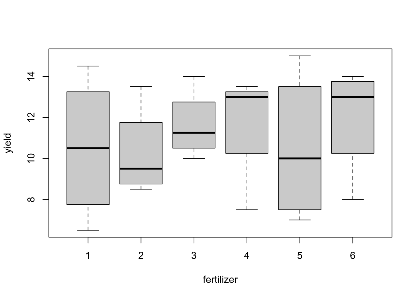
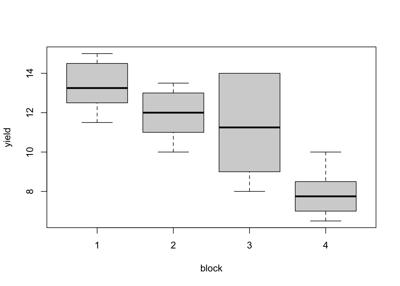
Figure 3.3: Blackcurrent experiment: yield against treatment and block.
There are substantial differences in average responses between blocks; differences between treatment means are smaller. These plots are only meaningful because this design is an RCBD, and each treatment occurs in each block.
The unit-block-treatment model is additive; that is, we assume the effect of each treatment does not vary for each block. Therefore we also need to check that there are no substantive interactions between treatments and blocks. We will do this graphically.
with(blackcurrent,
  interaction.plot(fertilizer, block, yield, xlab = 'Treatment', ylab = 'Yield', trace.label = 'Block')
)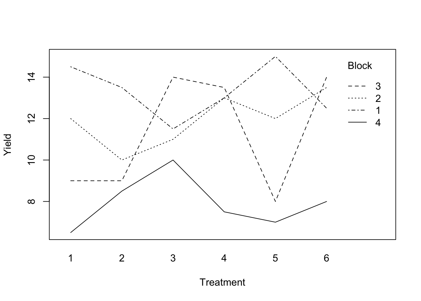
Figure 3.4: Blackcurrent experiment: treatment-block interaction plot.
Figure 3.4 plots the treatment means within each block. While there are clear differences between blocks, the differences between treatments do not seem to vary systematically between blocks.
We now fit a linear model, and perform an F-test for the hypothesis \(H_0: \tau_1 = \tau_2 = \tau_3 = \tau_4 = \tau_5 = \tau_6 = 0\).
## Analysis of Variance Table
##
## Response: yield
##            Df Sum Sq Mean Sq F value Pr(>F)
## block       3   94.9   31.62    8.90 0.0013 **
## fertilizer  5   11.8    2.36    0.66 0.6564
## Residuals  15   53.3    3.55
## ---
## Signif. codes:  0 '***' 0.001 '**' 0.01 '*' 0.05 '.' 0.1 ' ' 1
The “treatment” row of the ANOVA table compares the model including blocks and treatments to that only containing blocks. This comparison tests the above null hypothesis. We can see here that there is no evidence to reject \(H_0\) (p-value = 0.6564). This outcome is not surprising, given the tabular and graphical summaries we saw above. The block sum of squares is large, but we do not perform formal hypothesis testing for blocks.
Out of curiousity, we can also assess the “efficiency” of blocking by comparing the estimate of \(\sigma^2\) from the block design with the estimate that would result from ignoring the blocks, treating the experiment as a CRD and fitting a unit-treatment model.
blackcurrent_crd.lm <- lm(yield ~ fertilizer, data = blackcurrent)
summary(blackcurrent_crd.lm)$sig^2 / summary(blackcurrent.lm)$sig^2
## [1] 2.316The estimate of \(\sigma^2\) from the CRD is more the two times greater than the estimate from the block design, meaning about 100% more observations would be needed in the CRD to get the same level of precision as the RCBD.
We now examine residual diagnostics, to check the assumptions of our model:
- constant variance, with respect to the mean response, the treatment and the block
- normality of residuals
- additive treatment and block effects (already assessed in Fig 3.4).
standres <- rstandard(blackcurrent.lm)
fitted <- fitted(blackcurrent.lm)
par(mfrow = c(1, 3), pty = "s")
with(blackcurrent, {
  plot(fertilizer, standres, xlab = "Treatment", ylab = "Standarised residuals")
  plot(block, standres, xlab = "Block", ylab = "Standarised residuals")
  plot(fitted, standres, xlab = "Fitted value", ylab = "Standarised residuals")
})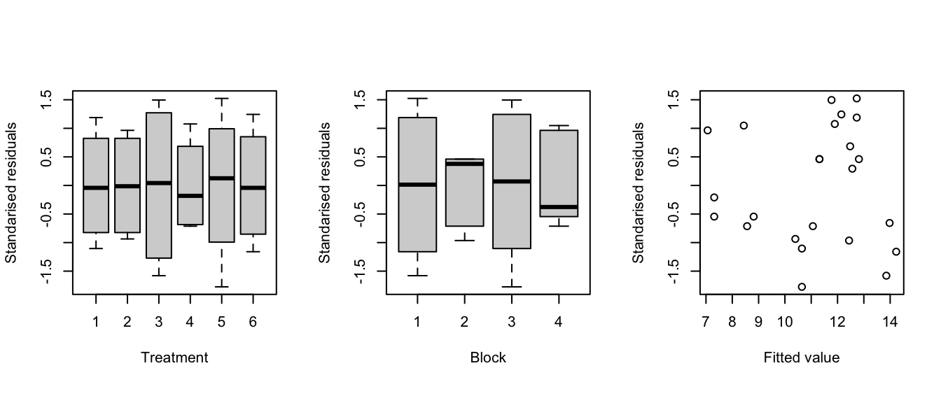
Figure 3.5: Blackcurrent experiment: Residuals against treatments (left), blocks (middle) and fitted values (right).
The plots in Figure 3.5 do not show any serious evidence of non-constant variance (maybe very slightly for blocks), and no large outliers.
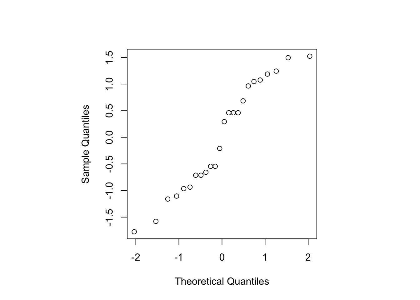
Figure 3.6: Blackcurrent experiment: Normal probability plot for standardised residuals.
Figure 3.6 shows the residuals lie roughly on a straight line when plotted against theoretical normal quantiles, and hence the assumption of normally distributed errors seems reasonable.
There is no evidence of a difference between treatments, so we would not normally test each pairwise difference. However, if we did, we could use the following code.
##  contrast                  estimate   SE df t.ratio p.value
##  fertilizer1 - fertilizer2    0.250 1.33 15   0.188  1.0000
##  fertilizer1 - fertilizer3   -1.125 1.33 15  -0.844  0.9541
##  fertilizer1 - fertilizer4   -1.250 1.33 15  -0.938  0.9303
##  fertilizer1 - fertilizer5    0.000 1.33 15   0.000  1.0000
##  fertilizer1 - fertilizer6   -1.500 1.33 15  -1.125  0.8635
##  fertilizer2 - fertilizer3   -1.375 1.33 15  -1.031  0.9000
##  fertilizer2 - fertilizer4   -1.500 1.33 15  -1.125  0.8635
##  fertilizer2 - fertilizer5   -0.250 1.33 15  -0.188  1.0000
##  fertilizer2 - fertilizer6   -1.750 1.33 15  -1.313  0.7741
##  fertilizer3 - fertilizer4   -0.125 1.33 15  -0.094  1.0000
##  fertilizer3 - fertilizer5    1.125 1.33 15   0.844  0.9541
##  fertilizer3 - fertilizer6   -0.375 1.33 15  -0.281  0.9997
##  fertilizer4 - fertilizer5    1.250 1.33 15   0.938  0.9303
##  fertilizer4 - fertilizer6   -0.250 1.33 15  -0.188  1.0000
##  fertilizer5 - fertilizer6   -1.500 1.33 15  -1.125  0.8635
##
## Results are averaged over the levels of: block
## P value adjustment: tukey method for comparing a family of 6 estimates
- Construct a BIBD for \(t=5\) treatments in \(b=5\) blocks of size \(k=4\) units. What are \(r\) and \(\lambda\) for your design? Compare your design to a RCBD via the efficiency for estimating a pairwise treatment difference.
Solution
Here, \(b = {t \choose k} = {5 \choose 4} = 5\), and hence we can use the “naive” construction method from the notes, where we can form one block from each possible subset of \(k=4\) treatments. This design will have \(r = {4 \choose 3} = 4\) and \(\lambda = {3 \choose 2} = 3\).
bibd <- t(combn(1:5, 4))
rownames(bibd) <- paste("Block", 1:5)
knitr::kable(bibd, caption = "BIBD for $t = 5$ treatments in $b=5$ blocks of size $k=4$.")| Block 1 | 1 | 2 | 3 | 4 |
| Block 2 | 1 | 2 | 3 | 5 |
| Block 3 | 1 | 2 | 4 | 5 |
| Block 4 | 1 | 3 | 4 | 5 |
| Block 5 | 2 | 3 | 4 | 5 |
The efficiency of this BIBD compared to a RCBD with \(b=5\) blocks of size \(k=5\) is given by \(\frac{\lambda t}{kb} = 0.75\). So variances will be 25% larger under the BIBD.
Consider an experiment for testing the abrasion resistance of rubber-coated fabric. There are four types of material, denoted A - D. The response is the loss in weight in 0.1 milligrams (mg) over a standard period of time. The testing machine has four positions, so four samples of material can be tested at a time. Past experience suggests that there may be differences between these positions, and there may be differences between each application of the testing machine (due to changes in set-up). Therefore, we have two blocking variables, “Position” and “Application”. For this experiment, we use a latin square design, as follows.
fabric <- data.frame(material = factor(c('C', 'D', 'B', 'A', 'A', 'B', 'D', 'C',
                           'D', 'C', 'A', 'B', 'B', 'A', 'C', 'D')),
               position = rep(factor(1:4), 4),
               application = rep(factor(1:4), rep(4, 4)),
               weight = c(235, 236, 218, 268,
                            251, 241, 227, 229,
                            234, 273, 274, 226,
                            195, 270, 230, 225)
                 )
knitr::kable(
 tidyr::pivot_wider(fabric, id_cols = application, names_from = position,
                values_from = material),
 col.names = c("Application", paste("Position", 1:4)))
Application Position 1 Position 2 Position 3 Position 4 1 C D B A 2 A B D C 3 D C A B 4 B A C D The blocking variables are represented as the rows and columns of the square; the latin letters represent the different treatments. A latin square of order \(k\) is a \(k\times k\) square of \(k\) latin letters arranged so that each letter appears exactly once in each row and column (Sudoko squares are also examples of latin squares). To perform the experiment, the levels of the blocking factors are randomly assigned to the rows and the columns, and the different treatments to the letters. A latin square design is a special case of the more general class of row column designs for two blocking factors.
A suitable unit-block-treatment model for a latin square design has the form
\[ y_{ijk} = \mu + \beta_i + \gamma_j + \tau_k + \varepsilon_{ijk}\,,\qquad i,j,k = 1,\ldots, t\,, \]
with \(\mu\) a constant parameter, \(\beta_i\) row block effects, \(\gamma_j\) column block effects and \(\tau_k\) the treatment effects. As usual, \(\varepsilon_{ijk}\sim N(0, \sigma^2)\), with errors from different units assumed independent. Note that not all combinations of \(i,j,k\) actually occur in the design; at the intersection of the \(i\)th row and \(j\)th column, only one of the \(t\) treatments is applied.
Write down a set of normal equations for the model parameters.
It can be shown that the reduced normal equations for the treatment parameters \(\tau_1,\ldots, \tau_t\) have the form \[ \hat{\tau}_k - \hat{\tau}_w = \bar{y}_{..j} - \bar{y}_{...}\,, \] with \(\hat{\tau}_w = \frac{1}{t}\sum_{k=1}^t\hat{\tau}_k\), \(\bar{y}_{..k} = \frac{1}{t}\sum_{i=1}^t\sum_{j=1}^tn_{ijk}y_{ijk}\) (mean for treatment \(k\)) and \(\bar{y}_{...} = \frac{1}{n}\sum_{i=1}^t\sum_{j=1}^t\sum_{k=1}^tn_{ij}y_{ijk}\) (overall mean) where \(n_{ijk} = 1\) if treatment \(k\) occurs at the intersection of row \(i\) and column \(j\) and zero otherwise, and \(\sum_{i=1}^t\sum_{j=1}^tn_{ijk} = t\) for all \(k=1, \ldots, t\).
Demonstrate that any contrast can therefore be estimated from this design, and derive the variance of the estimator of \(\sum_{k=1}^tc_k\tau_k\).
The data for this experiment is as follows, where the entries in the table give the response for the corresponding treatment:
knitr::kable(
 tidyr::pivot_wider(fabric, id_cols = application, names_from = position,
                values_from = weight),
 col.names = c("Application", paste("Position", 1:4)))
Application Position 1 Position 2 Position 3 Position 4 1 235 236 218 268 2 251 241 227 229 3 234 273 274 226 4 195 270 230 225 - For this data, test if there is a significant difference between materials. If there is, conduct multiple comparisons of all pairs at an experimentwise type I error rate of 5%.
Solution
We start by writing the model in matrix form:
\[\begin{align*} \boldsymbol{y}& = \boldsymbol{1}_n\mu + X_1\boldsymbol{\beta} + X_2\boldsymbol{\gamma} + X_3\boldsymbol{\tau} + \boldsymbol{\varepsilon}\\ & = W\boldsymbol{\alpha} + \boldsymbol{\varepsilon}\,, \end{align*}\]
with \(W = (\boldsymbol{1}_n, X_1, X_2, X_3)\), \(X_1\), \(X_2\) and \(X_3\) being \(n \times t\) model matrices for row blocks, column blocks and treatments, respectively, \(\boldsymbol{\alpha}^{\mathrm{T}} = (\mu, \boldsymbol{\beta}^{\mathrm{T}}, \boldsymbol{\gamma}^{\mathrm{T}}, \boldsymbol{\tau}^{\mathrm{T}})\) being a \((1+3t)\)-vector of parameters, and \(\boldsymbol{\varepsilon}\sim N(\boldsymbol{0}_n, I_n\sigma^2)\).
The normal equations are given by \(W^{\mathrm{T}}W\hat{\boldsymbol{\alpha}} = W^{\mathrm{T}}\boldsymbol{y}\), which can be expanded out to give the following four matrix equations:
\[\begin{align} n\hat{\mu} + \boldsymbol{1}_n^{\mathrm{T}}X_1\hat{\boldsymbol{\beta}} + \boldsymbol{1}_n^{\mathrm{T}}X_2\hat{\boldsymbol{\gamma}} + \boldsymbol{1}_n^{\mathrm{T}}X_3\hat{\boldsymbol{\tau}} & = \boldsymbol{1}_n^{\mathrm{T}}\boldsymbol{y}\,, \tag{3.16}\\ X_1^{\mathrm{T}}\boldsymbol{1}_n\hat{\mu} + X_1^{\mathrm{T}}X_1\hat{\boldsymbol{\beta}} + X_1^{\mathrm{T}}X_2\hat{\boldsymbol{\gamma}} + X_1^{\mathrm{T}}X_3\hat{\boldsymbol{\tau}} & = X_1^{\mathrm{T}}\boldsymbol{y}\,, \tag{3.17}\\ X_2^{\mathrm{T}}\boldsymbol{1}_n\hat{\mu} + X_2^{\mathrm{T}}X_1\hat{\boldsymbol{\beta}} + X_2^{\mathrm{T}}X_2\hat{\boldsymbol{\gamma}} + X_2^{\mathrm{T}}X_3\hat{\boldsymbol{\tau}} & = X_2^{\mathrm{T}}\boldsymbol{y}\,, \tag{3.18}\\ X_3^{\mathrm{T}}\boldsymbol{1}_n\hat{\mu} + X_3^{\mathrm{T}}X_1\hat{\boldsymbol{\beta}} + X_3^{\mathrm{T}}X_2\hat{\boldsymbol{\gamma}} + X_3^{\mathrm{T}}X_3\hat{\boldsymbol{\tau}} & = X_3^{\mathrm{T}}\boldsymbol{y}\,. \tag{3.19}\\ \end{align}\]
From the reduced normal equations given in the question, we have
\[\begin{align*} \sum_{k=1}^tc_k\left(\hat{\tau}_k - \hat{\tau}_w\right) & = \sum_{k=1}^tc_k\hat{\tau}_k \\ & = \sum_{k=1}^tc_k\left(\bar{y}_{..k} - \bar{y}_{...}\right) \\ & = \sum_{k=1}^tc_k\bar{y}_{..k}\,, \end{align*}\]
as \(\sum_{k=1}^tc_k\hat{\tau}_w = \sum_{k=1}^tc_k\bar{y}_{...} = 0\), as neither \(\hat{\tau}_w\) or \(\bar{y}_{...}\) depend on \(k\). Hence,
\[ \widehat{\boldsymbol{c}^{\mathrm{T}}\boldsymbol{\tau}} = \sum_{k=1}^tc_k\bar{y}_{..k}\,. \]
Or notice that the reduced normal equations for this design are the same as for a CRD with each treatment replicated \(t\) times.
We conduct these hypothesis tests using
R.## Analysis of Variance Table ## ## Response: weight ## Df Sum Sq Mean Sq F value Pr(>F) ## position 3 1468 489 7.99 0.01617 * ## application 3 986 329 5.37 0.03901 * ## material 3 4622 1540 25.15 0.00085 *** ## Residuals 6 368 61 ## --- ## Signif. codes: 0 '***' 0.001 '**' 0.01 '*' 0.05 '.' 0.1 ' ' 1The “material” line of the ANOVA table compares the models with and without the effects for material (but both models including the blocking factors). There is clearly a significant effect of material.
fabric.emm <- emmeans::emmeans(fabric.lm, ~ material)
fabric.pairs <- transform(pairs(fabric.emm))
dplyr::mutate(fabric.pairs, reject = p.value < 0.05)
## contrast estimate SE df t.ratio p.value reject ## 1 A - B 45.75 5.534 6 8.267 0.000703 TRUE ## 2 A - C 24.00 5.534 6 4.337 0.019036 TRUE ## 3 A - D 35.25 5.534 6 6.370 0.002866 TRUE ## 4 B - C -21.75 5.534 6 -3.930 0.029477 TRUE ## 5 B - D -10.50 5.534 6 -1.897 0.320631 FALSE ## 6 C - D 11.25 5.534 6 2.033 0.274277 FALSE
Using an experiment-wise error rate of 5%, we see significant differences between materials A and B, A and C, A and D, and B and C.
References
The four coatings were all made from Engineering Thermoplastic Polyurethane (ETPU); coating one was solely made from ETPU, coatings 2-4 had additional glass fibre, carbon fibre or aramid fibre added, respectively.↩︎
This is our first example of (partial) confounding, which we will see again in Chapters 5 and 6↩︎
Randanovadon’t, of course, know that this is a block design or that a blocking factor is being tested.↩︎These contrasts measure the difference between the coating only made from ETPU and the three coatings with added fibres.↩︎
Of course, the CRD has seven more degrees of freedom for estimating \(\sigma^2\) as block effects do not require estimation.↩︎