Chapter 1 Motivation, introduction and revision

Definition 1.1 An experiment is the process through which data are collected to answer a scientific question (physical science, social science, actuarial science \(\dots\)) by deliberately varying some features of the process under study in order to understand the impact of these changes on measureable responses.

In this course we consider only intervention experiments, in which some aspects of the process are under the experimenters’ control. We do not consider surveys or observational studies.

Definition 1.2 Design of experiments is the topic in Statistics concerned with the selection of settings of controllable variables or factors in an experiment and their allocation to experimental units in order to maximise the effectiveness of the experiment at achieving its aim.

People have been designing experiments for as long as they have been exploring the natural world. Collecting empirical evidence is key for scientific development, as described in terms of clinical trials by xkcd:

Some notable milestones in the history of the design of experiments include:

• prior to the 20th century:
  • Francis Bacon (17th century; pioneer of the experimental methods)
  • James Lind (18th century; experiments to eliminate scurvy)
  • Charles Peirce (19th century; advocated randomised experiments and randomisation-based inference)
• 1920s: agriculture (particularly at the Rothamsted Agricultural Research Station)
• 1940s: clinical trials (Austin Bradford-Hill)
• 1950s: (manufacturing) industry (W. Edwards Deming; Genichi Taguchi)
• 1960s: psychology and economics (Vernon Smith)
• 1980s: in-silico (computer experiments)
• 2000s: online (A/B testing)

See Luca and Bazerman (2020) for further history, anecdotes and examples, especially from psychology and technology.

Figure 1.1 shows the Broadbalk agricultural field experiment at Rothamsted, one of the longest continuous running experiments in the world, which is testing the impact of different manures and fertilizers on the growth of winter wheat.

Figure 1.1: The Broadbalk experiment, Rothamsted (photograph taken 2016)

1.1 Motivation

Example 1.1 Consider an experiment to compare two treatments (e.g. drugs, diets, fertilisers, \(\dots\)). We have \(n\) subjects (people, mice, plots of land, \(\dots\)), each of which can be assigned one of the two treatments. A response (protein measurement, weight, yield, \(\dots\)) is then measured.

Question: How many subjects should be assigned to each treatment to gain the most precise¹ inference about the difference in response from the two treatments?

Consider a linear statistical model² for the response (see MATH2010 or MATH6174/STAT6123):

\[\begin{equation} Y_j=\beta_{0}+\beta_{1}x_j+\varepsilon_j\,,\qquad j=1, \ldots, n\,, \tag{1.1} \end{equation}\]

where \(\varepsilon_j\sim N(0,\sigma^{2})\) are independent and identically distributed errors and \(\beta_{0}, \beta_{1}\) are unknown constants (parameters).

Let³ \[\begin{equation} x_{j}=\left\{\begin{array}{cl} 0&\textrm{if treatment 1 is applied to the $j$th subject}\\ 1&\textrm{if treatment 2 is applied to the $j$th subject}\nonumber , \end{array} \right. \end{equation}\] for \(j=1,\dots,n\).

The difference in expected response from treatments 1 and 2 is

\[\begin{equation} \begin{split} \textrm{E}[Y_j\, |\, x_j = 1] - \textrm{E}[Y_j\, |\, x_j = 0] & = \beta_{0}+\beta_{1}-\beta_{0} \\ & = \beta_{1}\,. \end{split} \tag{1.2} \end{equation}\]

Therefore, we require the the most precise estimator of \(\beta_{1}\) possible. That is, we wish to make the variance of our estimator of \(\beta_1\) as small as possible.

Parameters \(\beta_{0}\) and \(\beta_{1}\) can be estimated using least squares (see MATH2010 or MATH6174/STAT6123). For \(Y_1,\dots,Y_n\), we can write the model down in matrix form:

\[\begin{equation*} \left[ \begin{array}{c} Y_1\\ \vdots\\ Y_n\end{array}\right] =\left[ \begin{array}{cc} 1&x_{1}\\ \vdots&\vdots\\ 1&x_{n}\end{array}\right] \left[ \begin{array}{c} \beta_{0}\\ \beta_{1}\end{array}\right] +\left[ \begin{array}{c} \varepsilon_{1}\\ \vdots\\ \varepsilon_{n}\end{array}\right]\,. \end{equation*}\]

Or, by defining some notation:

\[\begin{equation} \boldsymbol{Y}=X\boldsymbol{\beta}+\boldsymbol{\varepsilon}\, \tag{1.3} \end{equation}\]

where

• \(\boldsymbol{Y}\) - \(n\times 1\) vector of responses;
• \(X\) - \(n\times p\) model matrix;
• \(\boldsymbol{\beta}\) - \(p\times 1\) vector of parameters;
• \(\boldsymbol{\varepsilon}\) - \(n\times 1\) vector of errors.

The least squares estimators, \(\hat{\boldsymbol{\beta}}\), are chosen such that the quadratic form

\[\begin{equation*} (\boldsymbol{Y}-X\boldsymbol{\beta})^{\textrm{T}}(\boldsymbol{Y}-X\boldsymbol{\beta}) \end{equation*}\]

is minimised (recall that \(\textrm{E}(\textbf{Y})=X\boldsymbol{\beta}\)). Therefore

\[\begin{equation*} \hat{\boldsymbol{\beta}} = \textrm{argmin}_{\boldsymbol{\beta}}(\boldsymbol{Y}^{\textrm{T}}\boldsymbol{Y}+\boldsymbol{\beta}^{\textrm{T}}X^{\textrm{T}}X\boldsymbol{\beta} -2\boldsymbol{\beta}^{\textrm{T}}X^{\textrm{T}}\boldsymbol{Y})\,. \end{equation*}\]

If we differentiate with respect to \(\boldsymbol{\beta}\)⁴,

\[\begin{equation*} \frac{\partial}{\partial\boldsymbol{\beta}}=2X^{\textrm{T}}X\boldsymbol{\beta}-2X^{\textrm{T}}\boldsymbol{Y}\,,\nonumber \end{equation*}\]

and equate to 0, we get the estimators

\[\begin{equation} \hat{\boldsymbol{\beta}}=(X^{\textrm{T}}X)^{-1}X^{\textrm{T}}\boldsymbol{Y}\,. \tag{1.4} \end{equation}\]

These are the least squares estimators.

For Example 1.1,

\[ X=\left[\begin{array}{cc} 1&x_{1}\\ \vdots&\vdots\\ 1&x_{n}\end{array}\right]\,, \qquad X^{\textrm{T}}X=\left[\begin{array}{cc} n&\sum x_j\\ \sum x_j&\sum x_j^{2}\end{array}\right]\,, \]

\[ (X^{\textrm{T}}X)^{-1}=\frac{1}{n\sum x_j^{2}-(\sum x_j)^{2}}\left[\begin{array}{cc} \sum x_j^{2}&-\sum x_j\\ -\sum x_j&n\end{array}\right]\,, \qquad X^{\textrm{T}}\boldsymbol{Y}=\left[\begin{array}{c} \sum Y_j\\ \sum x_jY_j\end{array}\right]\,. \] Then, \[\begin{align} \hat{\boldsymbol{\beta}}=\left[\begin{array}{c} \hat{\beta}_{0}\\ \hat{\beta}_{1}\end{array}\right] & =\frac{1}{n\sum x_j^{2}-(\sum x_j)^{2}} \left[\begin{array}{cc} \sum x_j^{2}&-\sum x_j\\ -\sum x_j&n\end{array}\right] \left[\begin{array}{c} \sum Y_j\\ \sum x_jY_j\end{array}\right]\nonumber \\ &= \frac{1}{n\sum x_j^{2}-(\sum x_j)^{2}}\left[\begin{array}{c} \sum Y_j\sum x_j^{2}-\sum x_j\sum x_jY_j\\ n\sum x_jY_j-\sum x_j\sum Y_j\end{array}\right]\,. \end{align}\]

We don’t usually work through the algebra in such detail; the matrix form is often sufficient for theoretical and numerical calculations and software, e.g. R, can be used.

The precision of \(\hat{\boldsymbol{\beta}}\) is measured via the variance-covariance matrix, given by \[\begin{align} \textrm{Var}(\hat{\boldsymbol{\beta}}) & = \textrm{Var}\{(X^{\textrm{T}}X)^{-1}X^{\textrm{T}}\boldsymbol{Y}\}\\ & =(X^{\textrm{T}}X)^{-1}X^{\textrm{T}}\textrm{Var}(\boldsymbol{Y})X(X^{\textrm{T}}X)^{-1}\\ & = (X^{\textrm{T}}X)^{-1}\sigma^{2}\,, \end{align}\]

where \(\boldsymbol{Y}\sim N(X\boldsymbol{\beta},I_n\sigma^{2})\), where \(I_n\) is an \(n\times n\) identity matrix.

Hence, in our example, \[\begin{align*} \textrm{Var}(\hat{\boldsymbol{\beta}}) & = \frac{1}{n\sum x_j^{2}-(\sum x_j)^{2}}\left[\begin{array}{cc} \sum x_j^{2}&-\sum x_j\\ -\sum x_j&n\end{array}\right]\sigma^{2}\\ & = \left[\begin{array}{cc} \textrm{Var}(\hat\beta_{0})&\textrm{Cov}(\hat\beta_{0},\hat\beta_{1})\\ \textrm{Cov}(\hat\beta_{0},\hat\beta_{1})&\textrm{Var}(\hat\beta_{1})\end{array}\right]\,. \end{align*}\]

For estimating the difference between treatments, we are interested in

\[\begin{align*} \textrm{Var}(\hat{\beta}_{1})& = \frac{n}{n\sum x_j^{2}-(\sum x_j)^{2}}\sigma^{2}\\ & = \frac{1}{\sum x_j^{2} - n\bar{x}^2}\sigma^{2}\,, \end{align*}\] where \(\bar{x} = \sum x_j / n\).

Assuming constant \(\sigma^2\), to achieve the most precise estimator we need to minimise \(\textrm{Var}(\hat{\beta}_{1})\) or equivalently maxmise \(\sum x_j^{2} - n\bar{x}^2\). This goal can be achieved through the choice of \(x_{1},\dots,x_{n}\):

• as each \(x_j\) can only take one of two values, 0 or 1, this is equivalent to choosing the numbers of subjects assigned to treatment 1 and treatment 2;
• call these \(n_{1}\) and \(n_{2}\) respectively, with \(n_{1}+n_{2}=n\).

We can find an upper bound for the quantity \(\sum x_j^{2} - n\bar{x}^2\). As each \(x_i\in\{0,1\}\) we have

\[\begin{align} \sum x_j^2 & = \sum x_j \\ & = n\bar{x}\,. \end{align}\]

Hence,

\[\begin{align*} \sum x_j^{2} - n\bar{x}^2 & = n\bar{x} - n\bar{x}^2 \\ & = n\bar{x}(1-\bar{x}) \\ & \le n/4\,, \end{align*}\] as we have a quadratic equation in \(\bar{x}\) that is maximised at \(\bar{x} = 1/2\).

If we can find a set of design points that satisfy \(\bar{x} = 1/2\), we will have an optimal design. Assuming \(n\) is even, one possibility is

• \(n_{1}=\frac{n}{2}\) subjects assigned to treatment 1 (\(x_j = 0\)) and
• \(n_{2}=\frac{n}{2}\) subjects assigned to treatment 2 (\(x_j = 1\)).

For \(n\) odd, we choose \(n_{1}=\frac{n+1}{2}\), \(n_{2}=\frac{n-1}{2}\), or vice versa, to get as close as possible to the optimal design.

Definition 1.3 We can assess different designs using their efficiency: \[\begin{equation} \textrm{Eff}=\frac{\textrm{Var}(\hat{\beta}_{1}\, |\, d^{*})}{\textrm{Var}(\hat{\beta}_{1}\, |\, d_{1})} \tag{1.5} \end{equation}\]

where \(d_{1}\) is a design we want to assess and \(d^{*}\) is the optimal design with smallest variance. Note that \(0\leq\textrm{Eff}\leq 1\).

In Figure 1.2 below, we plot this efficiency for Example 1.1, using different choices of \(n_1\). The total number of runs is fixed at \(n = 100\), and the function eff calculates the efficiency (assuming \(n\) is even) from Definition 1.3 for a design with \(n_1\) subjects assigned to treatment 1. Clearly, efficiency of 1 is achieved when \(n_1 = n_2\) (equal allocation of treatments 1 and 2). If \(n_1=0\) or \(n_1 = 1\), the efficiency is zero; we cannot estimate the difference between two treatments if we only allocate subjects to one of them.

n <- 100
eff <- function(n2) 4 * n2 * (n - n2) / n^2
curve(eff, from = 0, to = n, ylab = "Eff", xlab = expression(n[1]))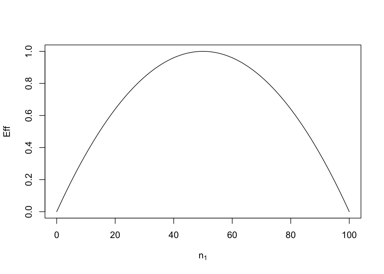

Figure 1.2: Efficiencies for designs for Example 1.1 with different numbers, \(n_1\), of subjects assigned to treatment 1 when the total number of subjects is \(n=100\).

1.2 Aims of experimentation and some examples

Some reasons experiments are performed:

1. Treatment comparison

• compare several treatments (and choose the best)
• e.g. clinical trial, agricultural field trial

2. Factor screening

• many complex systems may involve a large number of (discrete) factors (controllable features)
• which of these factors have a substantive impact?
• (relatively) small experiments
• e.g. industrial experiments on manufacturing processes

3. Response surface exploration

• detailed description of relationship between important (continuous) variables and response
• typically second order polynomial regression models
• larger experiments, often built up sequentially
• e.g. alcohol yields in a pharmaceutical experiments

4. Optimisation

• finding settings of variables that lead to maximum or minimum response
• typically use response surface methods and sequential “hill climbing” strategy

In this module, we will focus on treatment comparison (Chapters 2 and 3) and factor screening (Chapters 4, 5 and 6).

1.3 Some definitions

Definition 1.4 The response \(Y\) is the outcome measured in an experiment; e.g. yield from a chemical process. The response from the \(n\) observations are denoted \(Y_{1},\dots,Y_{n}\).

Definition 1.5 Factors (discrete) or variables (continuous) are features which can be set or controlled in an experiment; \(m\) denotes the number of factors or variables under investigation. For discrete factors, we call the possible settings of the factor its levels. We denote by \(x_{ij}\) the value taken by factor or variable \(i\) in the \(j\)th run of the experiment (\(i = 1, \ldots, m\); \(j = 1, \ldots, n\)).

Definition 1.6 The treatments or support points are the distinct combinations of factor or variable values in the experiment.

Definition 1.7 An experimental unit is the basic element (material, animal, person, time unit, ) to which a treatment can be applied to produce a response.

In Example 1.1 (comparing two treatments):

• Response \(Y\): Measured outcome, e.g. protein level or pain score in clinical trial, yield in an agricultural field trial.
• Factor \(x\): “treatment” applied
• Levels \[ \begin{array}{ll} \textrm{treatment 1}&x =0\\ \textrm{treatment 2}&x =1 \end{array} \]
• Treatment or support point: Two treatments or support points
• Experimental unit: Subject (person, animal, plot of land, \(\ldots\)).

1.4 Principles of experimentation

Three fundamental principles that need to be considered when designing an experiment are:

• replication
• randomisation
• stratification (blocking)

1.4.1 Replication

Each treatment is applied to a number of experimental units, with the \(j\)th treatment replicated \(r_{j}\) times. This enables the estimation of the variances of treatment effect estimators; increasing the number of replications, or replicates, decreases the variance of estimators of treatment effects. (Note: proper replication involves independent application of the treatment to different experimental units, not just taking several measurements from the same unit).

1.4.2 Randomisation

Randomisation should be applied to the allocation of treatments to units. Randomisation protects against bias; the effect of variables that are unknown and potentially uncontrolled or subjectivity in applying treatments. It also provides a formal basis for inference and statistical testing.

For example, in a clinical trial to compare a new drug and a control random allocation protects against

• “unmeasured and uncontrollable” features (e.g. age, sex, health)
• bias resulting from the clinician giving new drug to patients who are sicker.

Clinical trials are usually also double-blinded, i.e. neither the healthcare professional nor the patient knows which treatment the patient is receiving.

1.4.3 Stratification (or blocking)

We would like to use a wide variety of experimental units (e.g. people or plots of land) to ensure coverage of our results, i.e. validity of our conclusions across the population of interest. However, if the sample of units from the population is too heterogenous, then this will induce too much random variability, i.e. increase \(\sigma^{2}\) in \(\varepsilon_{j}\sim N(0,\sigma^{2})\), and hence increase the variance of our parameter estimators.

We can reduce this extraneous variation by splitting our units into homogenous sets, or blocks, and including a blocking term in the model. The simplest blocked experiment is a randomised complete block design, where each block contains enough units for all treatments to be applied. Comparisons can then be made within each block.

Basic principle: block what you can, randomise what you cannot.

Later we will look at blocking in more detail, and the principle of incomplete blocks.

1.5 Revision on the linear model

Recall: \(\boldsymbol{Y}=X\boldsymbol{\beta}+\boldsymbol{\varepsilon}\), with \(\boldsymbol{\varepsilon}\sim N(\boldsymbol{0},I_n\sigma^{2})\). Let the \(j\)th row of \(X\) be denoted \(\boldsymbol{x}^\textrm{T}_j\), which holds the values of the predictors, or explanatory variables, for the \(j\)th observation. Then

\[\begin{equation*} Y_j=\boldsymbol{x}_j^{\textrm{T}}\boldsymbol{\beta}+\varepsilon_j\,,\quad j=1,\ldots,n\,. \end{equation*}\]

For example, quite commonly, for continuous variables

\[ \boldsymbol{x}_j=(1,x_{1j},x_{2j},\dots,x_{mj})^{\textrm{T}}\,, \]

and so \[ \boldsymbol{x}_j^{\textrm{T}}\boldsymbol{\beta}=\beta_{0}+\beta_{1}x_{1j}+\dots+\beta_{m}x_{mj}\,. \]

The least squares estimators are given by

\[\begin{equation} \hat{\boldsymbol{\beta}}=(X^{\textrm{T}}X)^{-1}X^{\textrm{T}}\boldsymbol{Y}\,,\nonumber \end{equation}\]

with

\[\begin{equation} \textrm{Var}(\hat{\boldsymbol{\beta}})=(X^{\textrm{T}}X)^{-1}\sigma^{2}\,.\nonumber \end{equation}\]

1.5.1 Analysis of Variance as Model Comparison

To assess the goodness-of-fit of a model, we can use the residual sum of squares

\[\begin{align*} \textrm{RSS} & = (\boldsymbol{Y} - X\hat{\boldsymbol{\beta}})^{\textrm{T}} (\boldsymbol{Y} - X\hat{\boldsymbol{\beta}})\\ & = \sum^{n}_{j=1}\left\{Y_{j}-\boldsymbol{x}_{j}^{\textrm{T}}\hat{\boldsymbol{\beta}}\right\}^{2}\\ & = \sum^{n}_{j=1}r_{j}^{2}\,, \end{align*}\]

where

\[ r_{j}=Y_{j}-\boldsymbol{x}_{j}^{\textrm{T}}\hat{\boldsymbol{\beta}}\,. \]

Often, a comparison is made to the null model

\[ Y_{j}=\beta_{0}+\varepsilon_{j}\,, \]

i.e. \(Y_{i}\sim N(\beta_{0},\sigma^{2})\). The residual sum of squares for the null model is given by

\[ \textrm{RSS}(\textrm{null}) = \boldsymbol{Y}^{\textrm{T}}\boldsymbol{Y} - n\bar{Y}^{2}\,, \] as

\[ \hat{\beta}_{0} = \bar{Y} = \frac{1}{n}\sum_{j=1}^n Y_{j}\,. \]

An Analysis of variance (ANOVA) table is compact way of presenting the results of (sequential) comparisons of nested models. You should be familiar with an ANOVA table of the following form.

Table 1.1: A standard ANOVA table.

Source	Degress of Freedom	(Sequential) Sum of Squares	Mean Square
Regression	\(p-1\)	By subtraction; see (1.6)	Reg SS/\((p-1)\)
Residual	\(n-p\)	\((\boldsymbol{Y}-X\hat{\boldsymbol{\beta}})^{\textrm{T}}(\boldsymbol{Y}-X\hat{\boldsymbol{\beta}})\)5	RSS/\((n-p)\)
Total	\(n-1\)	\(\boldsymbol{Y}^{\textrm{T}}\boldsymbol{Y}-n\bar{Y}^{2}\)6

In row 1 of Table 1.1 above, \[\begin{align} \textrm{Regression SS = Total SS $-$ RSS} & = \boldsymbol{Y}^{\textrm{T}}\boldsymbol{Y} - n\bar{Y}^{2} - (\boldsymbol{Y}-X\hat{\boldsymbol{\beta}})^{\textrm{T}}(\boldsymbol{Y}-X\hat{\boldsymbol{\beta}})\\ & = -n\bar{Y}^{2}-\hat{\boldsymbol{\beta}}^{\textrm{T}}(X^{\textrm{T}}X)\hat{\boldsymbol{\beta}}+2\hat{\boldsymbol{\beta}}^{\textrm{T}}X^{\textrm{T}}\boldsymbol{Y} \\ & = \hat{\boldsymbol{\beta}}^{\textrm{T}}(X^{\textrm{T}}X)\hat{\boldsymbol{\beta}}-n\bar{Y}^{2}\,, \tag{1.6} \end{align}\]

with the last line following from \[\begin{align*} \hat{\boldsymbol{\beta}}^{\textrm{T}}X^{\textrm{T}}\boldsymbol{Y} & = \hat{\boldsymbol{\beta}}^{\textrm{T}}(X^{\textrm{T}}X)(X^{\textrm{T}}X)^{-1}X^{\textrm{T}}\boldsymbol{Y} \\ & = \hat{\boldsymbol{\beta}}^{\textrm{T}}(X^{\textrm{T}}X)\hat{\boldsymbol{\beta}} \end{align*}\]

This idea can be generalised to the comparison of a sequence of nested models - see Problem Sheet 1.

Hypothesis testing is performed using the mean square:

\[\begin{equation} \frac{\textrm{Regression SS}}{p-1}=\frac{\hat{\boldsymbol{\beta}}^{\textrm{T}}(X^{\textrm{T}}X)\hat{\boldsymbol{\beta}}-n\bar{Y}^{2}}{p-1}\,.\nonumber \end{equation}\]

Under \(\textrm{H}_{0}: \beta_{1}=\dots=\beta_{p-1}=0\)

\[\begin{align*} \frac{\textrm{Regression SS}/(p-1)}{\textrm{RSS}/(n-p)} & = \frac{(\hat{\boldsymbol{\beta}}^{\textrm{T}}(X^{\textrm{T}}X)\hat{\boldsymbol{\beta}} - n\bar{Y}^{2})/(p-1)}{(\boldsymbol{Y}-X\hat{\boldsymbol{\beta}})^{\textrm{T}}(\boldsymbol{Y}-X\hat{\boldsymbol{\beta}})/(n-p)}\nonumber\\ & \sim F_{p-1,n-p}\,, \end{align*}\]

an \(F\) distribution with \(p-1\) and \(n-p\) degrees of freedom; defined via the ratio of two independent \(\chi^{2}\) distributions.

Also,

\[\begin{equation*} \frac{\textrm{RSS}}{n-p}=\frac{(\boldsymbol{Y}-X\hat{\boldsymbol{\beta}})^{\textrm{T}}(\boldsymbol{Y}-X\hat{\boldsymbol{\beta}})}{n-p}=\hat{\sigma}^{2} \end{equation*}\]

is an unbiased estimator for \(\sigma^{2}\), and

\[\begin{equation*} \frac{(n-p)}{\sigma^{2}}\hat{\sigma}^{2}\sim\chi^{2}_{n-p}\,. \end{equation*}\]

This is a Chi-squared distribution with \(n-p\) degrees of freedom (see MATH2010 or MATH6174 notes).

1.6 Exercises

1. (Adapted from Morris, 2011) A classic and famous example of a simple hypothetical experiment was described by Fisher (1935):

   A lady declares that by tasting a cup of tea made with milk she can discriminate whether the milk or the tea infusion was added first to the cup. We will consider the problem of designing an experiment by means of which this assertion can be tested. For this purpose let us first lay down a simple form of experiment with a view to studying its limitations and its characteristics, both those that same essential to the experimental method, when well developed, and those that are not essential but auxiliary.

   Our experiment consists in mixing eight cups of tea, four in one way and four in the other, and presenting them to the subject for judgement in a random order. The subject has been told in advance of what the test will consist, namely that she will be asked to taste eight cups, that these shall be four of each kind, and that they shall be presented to her in a random order, that is an order not determined arbitrarily by human choice, but by the actual manipulation of the physical appartatus used in games of chance, cards, dice, roulettes, etc., or, more expeditiously, from a published collection of random sampling numbers purporting to give the actual results of such manipulation⁷. Her task is to divide the 8 cups into two sets of 4, agreeing, if possible, with the treatments received.

   1. Define the treatments in this experiment.
   2. Identify the units in this experiment.
   3. How might a “physical appartatus” from a “game of chance” be used to perform the randomisation? Explain one example.
   4. Suppose eight tea cups are available for this experiment but they are not identical. Instead they come from two sets. Four are made from heavy, thick porcelain; four from much lighter china. If each cup can only be used once, how might this fact be incorporated into the design of the experiment?

Solution

1. There are two treatments in the experiment - the two ingredients “milk first” and “tea first”.

2. The experimental units are the “cups of tea”, made up from the tea and milk used and also the cup itself.

3. The simplest method here might be to select four black playing cards and four red playing cards, assign one treatment to each colour, shuffle the cards, and then draw them in order. The colour drawn indicates the treatment that should be used to make the next cup of tea. This operation would give one possible randomisation.

   We could of course also use R.

sample(rep(c("Milk first", "Tea first"), c(4, 4)), size = 8, replace = F)

## [1] "Milk first" "Tea first"  "Milk first" "Milk first" "Tea first" 
## [6] "Tea first"  "Tea first"  "Milk first"

4. Type of cup could be considered as a blocking factor. One way of incorporating it would be to split the experiment into two (blocks), each with four cups (two milk first, two tea first). We would still wish to randomise allocation of treatments to units within blocks.

    # block 1
    sample(rep(c("Milk first", "Tea first"), c(2, 2)), size = 4, replace = F)

## [1] "Milk first" "Milk first" "Tea first"  "Tea first"

    # block 2
    sample(rep(c("Milk first", "Tea first"), c(2, 2)), size = 4, replace = F)

## [1] "Milk first" "Milk first" "Tea first"  "Tea first"

2. Consider the linear model

   \[\boldsymbol{y}= X\boldsymbol{\beta}+ \boldsymbol{\varepsilon}\,,\] with \(\boldsymbol{y}\) an \(n\times 1\) vector of responses, \(X\) a \(n\times p\) model matrix and \(\boldsymbol{\varepsilon}\) a \(n\times 1\) vector of independent and identically distributed random variables with constant variance \(\sigma^2\).

   1. Derive the least squares estimator \(\hat{\boldsymbol{\beta}}\) for this multiple linear regression model, and show that this estimator is unbiased. Using the definition of (co)variance, show that

   \[\mbox{Var}(\hat{\boldsymbol{\beta}}) = \left(X^{\mathrm{T}}X\right)^{-1}\sigma^2\,.\]

   2. If \(\boldsymbol{\varepsilon}\sim N (\boldsymbol{0},I_n\sigma^2)\), with \(I_n\) being the \(n\times n\) identity matrix, show that the maximum likelihood estimators for \(\boldsymbol{\beta}\) coincide with the least squares estimators.

Solution

1. The method of least squares minimises the sum of squared differences between the responses and the expected values, that is, minimises the expression

   \[ (\boldsymbol{y}-X\boldsymbol{\beta})^{\mathrm{T}}(\boldsymbol{y}-X\boldsymbol{\beta}) = \boldsymbol{y}^{\mathrm{T}}\boldsymbol{y}- 2\boldsymbol{\beta}^{\mathrm{T}}X^{\mathrm{T}}\boldsymbol{y}+ \boldsymbol{\beta}^{\mathrm{T}}X^{\mathrm{T}}X\boldsymbol{\beta}\,. \] Differentiating with respect to the vector \(\boldsymbol{\beta}\), we obtain

   \[ \frac{\partial}{\partial\boldsymbol{\beta}} = -2X^{\mathrm{T}}\boldsymbol{y}+ 2X^{\mathrm{T}}X\boldsymbol{\beta}\,. \]

   Set equal to \(\boldsymbol{0}\) and solve:

   \[ X^{\mathrm{T}}X\hat{\boldsymbol{\beta}} = X^{\mathrm{T}}\boldsymbol{y}\Rightarrow \hat{\boldsymbol{\beta}} = \left(X^{\mathrm{T}}X\right)^{-1}X^{\mathrm{T}}\boldsymbol{y}\,. \]

   The estimator \(\hat{\boldsymbol{\beta}}\) is unbiased:

   \[ E(\hat{\boldsymbol{\beta}}) = \left(X^{\mathrm{T}}X\right)^{-1}X^{\mathrm{T}}E(\boldsymbol{y}) = \left(X^{\mathrm{T}}X\right)^{-1}X^{\mathrm{T}}X\boldsymbol{\beta}= \boldsymbol{\beta}\,, \]

   and has variance:

   \[\begin{align*} \mbox{Var}(\hat{\boldsymbol{\beta}}) & =E\left\{ \left[\hat{\boldsymbol{\beta}} - E(\hat{\boldsymbol{\beta}})\right] \left[\hat{\boldsymbol{\beta}} - E(\hat{\boldsymbol{\beta}})\right]^{\mathrm{T}} \right\}\\ & = E\left\{ \left[\hat{\boldsymbol{\beta}} - \boldsymbol{\beta}\right] \left[\hat{\boldsymbol{\beta}} - \boldsymbol{\beta}\right]^{\mathrm{T}} \right\}\\ & = E\left\{ \hat{\boldsymbol{\beta}}\hat{\boldsymbol{\beta}}^{\mathrm{T}} - 2\boldsymbol{\beta}\hat{\boldsymbol{\beta}}^{\mathrm{T}} + \boldsymbol{\beta}\boldsymbol{\beta}^{\mathrm{T}} \right\}\\ & = E\left\{ \left(X^{\mathrm{T}}X\right)^{-1}X^{\mathrm{T}}\boldsymbol{y}\boldsymbol{y}^{\mathrm{T}}X\left(X^{\mathrm{T}}X\right)^{-1} - 2\boldsymbol{\beta}\boldsymbol{y}^{\mathrm{T}}X\left(X^{\mathrm{T}}X\right)^{-1} + \boldsymbol{\beta}\boldsymbol{\beta}^{\mathrm{T}}\right\}\\ & = \left(X^{\mathrm{T}}X\right)^{-1}X^{\mathrm{T}}E(\boldsymbol{y}\boldsymbol{y}^{\mathrm{T}})X\left(X^{\mathrm{T}}X\right)^{-1} - 2\boldsymbol{\beta}E(\boldsymbol{y}^{\mathrm{T}})X\left(X^{\mathrm{T}}X\right)^{-1} + \boldsymbol{\beta}\boldsymbol{\beta}^{\mathrm{T}}\\ & = \left(X^{\mathrm{T}}X\right)^{-1}X^{\mathrm{T}}\left[\mbox{Var}(\boldsymbol{y}) + E(\boldsymbol{y})E(\boldsymbol{y}^{\mathrm{T}})\right]X\left(X^{\mathrm{T}}X\right)^{-1} - 2\boldsymbol{\beta}\boldsymbol{\beta}^{\mathrm{T}}X^{\mathrm{T}}X\left(X^{\mathrm{T}}X\right)^{-1} + \boldsymbol{\beta}\boldsymbol{\beta}^{\mathrm{T}}\\ & = \left(X^{\mathrm{T}}X\right)^{-1}X^{\mathrm{T}}\left[I_N\sigma^2 + X\boldsymbol{\beta}\boldsymbol{\beta}^{\mathrm{T}}X^{\mathrm{T}}\right]X\left(X^{\mathrm{T}}X\right)^{-1} - \boldsymbol{\beta}\boldsymbol{\beta}^{\mathrm{T}}\\ & = \left(X^{\mathrm{T}}X\right)^{-1}\sigma^2\,. \end{align*}\]

2. As \(\boldsymbol{y}\sim N\left(X\boldsymbol{\beta}, I_N\sigma^2\right)\), the likelihood is given by

   \[ L(\boldsymbol{\beta}\,; \boldsymbol{y}) = \left(2\pi\sigma^2\right)^{-N/2}\exp\left\{-\frac{1}{2\sigma^2}(\boldsymbol{y}- X\boldsymbol{\beta})^{\mathrm{T}}(\boldsymbol{y}- X\boldsymbol{\beta})\right\}\,. \]

   The log-likelihood is given by

   \[ l(\boldsymbol{\beta}\,;\boldsymbol{y}) = -\frac{1}{2\sigma^2}(\boldsymbol{y}- X\boldsymbol{\beta})^{\mathrm{T}}(\boldsymbol{y}- X\boldsymbol{\beta}) + \mbox{constant}\,. \]

   Up to a constant, this expression is \(-1\times\) the least squares equations; hence maximising the log-likelihood is equivalent to minimising the least squares equation.

3. Consider the two nested linear models

   1. \(Y_j = \beta_0 + \beta_1x_{1j} + \beta_2x_{2j} + \ldots + \beta_{p_1}x_{p_1j} + \varepsilon_j\), or \(\boldsymbol{y}= \boldsymbol{1}_n\beta_0 + X_1\boldsymbol{\beta}_1 + \boldsymbol{\varepsilon}\),

   2. \(Y_j = \beta_0 + \beta_1x_{1j} + \beta_2x_{2j} + \ldots + \beta_{p_1}x_{p_1j} + \beta_{p_1+1}x_{(p_1+1)j} + \ldots + \beta_{p_1+p_2}x_{p_1+p_2j} + \varepsilon_j\), or \(\boldsymbol{y}= \boldsymbol{1}_n\beta_0 + X_1\boldsymbol{\beta}_1 + X_2\boldsymbol{\beta}_2+ \boldsymbol{\varepsilon}\)

   with \(\varepsilon_j\sim N(0, \sigma^2)\), and \(\varepsilon_{j}\), \(\varepsilon_{k}\) independent \((\boldsymbol{\varepsilon}\sim N(\boldsymbol{0},I_n\sigma^2))\).

   1. Construct an ANOVA table to compare model (ii) with the null model \(Y_j=\beta_0 + \varepsilon_j\).

   2. Extend this ANOVA table to compare models (i) and (ii) by further decomposing the regression sum of squares for model (ii).

   Hint: which residual sum of squares are you interested in to compare models (i) and (ii)?

   You should end up with an ANOVA table of the form

   Source	Degrees of freedom	Sums of squares	Mean square
   Model (i)	\(p_1\)	?	?
   Model (ii)	\(p_2\)	?	?
   Residual	\(n-p_1-p_2-1\)	?	?
   Total	\(n-1\)	\(\boldsymbol{y}^{\mathrm{T}}\boldsymbol{y}- n\bar{Y}^2\)

   The second row of the table gives the extra sums of squares for the additional terms in fitting model (ii), over and above those in model (i).

   3. Calculate the extra sum of squares for fitting the terms in model (i), over and above those terms only in model (ii), i.e. those held in \(X_2\boldsymbol{\beta}_2\). Construct an ANOVA table containing both the extra sum of squares for the terms only in model (i) and the extra sum of squares for the terms only in model (ii). Comment on the table.

Solution

1. From lectures

   Source	Degrees of freedom	Sums of squares	Mean square
   Regression	\(p_1+p_2\)	\(\hat{\boldsymbol{\beta}}^{\mathrm{T}}X^{\mathrm{T}}X\hat{\boldsymbol{\beta}} - n\bar{Y}^2\)	\(\left(\hat{\boldsymbol{\beta}}^{\mathrm{T}}X^{\mathrm{T}}X\hat{\boldsymbol{\beta}} - n\bar{Y}^2\right)/(p_1+p_2)\)
   Residual	\(n-p_1-p_2-1\)	\((\boldsymbol{y}- X\hat{\boldsymbol{\beta}})^{\mathrm{T}}(\boldsymbol{y}- X\hat{\boldsymbol{\beta}})\)	RSS\(/(n-p_1-p_2-1)\)
   Total	\(n-1\)	\(\boldsymbol{y}^{\mathrm{T}}\boldsymbol{y}- n\bar{Y}^2\)

   where \(X = [\boldsymbol{1}_n\, X_1 \, X_2]\).

   \[\begin{align*} \mbox{RSS(null) - RSS(ii)} & = \boldsymbol{y}^{\mathrm{T}}\boldsymbol{y}- n\bar{Y}^2 - (\boldsymbol{y}- X\hat{\boldsymbol{\beta}})^{\mathrm{T}}(\boldsymbol{y}- X\hat{\boldsymbol{\beta}})\\ & = \boldsymbol{y}^{\mathrm{T}}\boldsymbol{y}- n\bar{Y}^2 - \boldsymbol{y}^{\mathrm{T}}\boldsymbol{y}+ 2\boldsymbol{y}^{\mathrm{T}}X\hat{\boldsymbol{\beta}} - \hat{\boldsymbol{\beta}}^{\mathrm{T}}X^{\mathrm{T}}X\hat{\boldsymbol{\beta}}\\ & = 2\hat{\boldsymbol{\beta}}^{\mathrm{T}}X^{\mathrm{T}}X\hat{\boldsymbol{\beta}} - \hat{\boldsymbol{\beta}}^{\mathrm{T}}X^{\mathrm{T}}X\hat{\boldsymbol{\beta}} - n\bar{Y}^2\\ & = \hat{\boldsymbol{\beta}}^{\mathrm{T}}X^{\mathrm{T}}X\hat{\boldsymbol{\beta}} - n\bar{Y}^2\,. \end{align*}\]

2. To compare model (i) with the null model, we compute

   \[\begin{align*} \mbox{RSS(null) - RSS(i)} & = \boldsymbol{y}^{\mathrm{T}}\boldsymbol{y}- N\bar{Y}^2 - (\boldsymbol{y}- X_1^*\hat{\boldsymbol{\beta}}_1^*)^{\mathrm{T}}(\boldsymbol{y}- X_1^*\hat{\boldsymbol{\beta}}_1^*)\\ & = (\hat{\boldsymbol{\beta}}_1^*)^{\mathrm{T}}(X_1^*)^{\mathrm{T}}X_1^*\hat{\boldsymbol{\beta}}_1^* - n\bar{Y}^2\,, \end{align*}\] where \(X_1^* = [\boldsymbol{1}\, X_1]\) and \(\boldsymbol{\beta}_1^* = (\beta_0, \boldsymbol{\beta}_1^{\mathrm{T}})^{\mathrm{T}}\).

   To compare models (i) and (ii), we compare them both to the null model, and look at the difference between these comparisons:

   \[\begin{align*} \mbox{[RSS(null) - RSS(ii)] - [RSS(null) - RSS(i)]} & = \mbox{RSS(i) - RSS(ii)}\\ & = (\boldsymbol{y}- X_1^*\hat{\boldsymbol{\beta}}_1^*)^{\mathrm{T}}(\boldsymbol{y}- X_1^*\hat{\boldsymbol{\beta}}_1^*) - (\boldsymbol{y}- X\hat{\boldsymbol{\beta}})^{\mathrm{T}}(\boldsymbol{y}- X\hat{\boldsymbol{\beta}})\\ & = \hat{\boldsymbol{\beta}}^{\mathrm{T}}X^{\mathrm{T}}X\hat{\boldsymbol{\beta}} - (\hat{\boldsymbol{\beta}}_1^*)^{\mathrm{T}}(X_1^*)^{\mathrm{T}}X_1^*\hat{\boldsymbol{\beta}}_1^*\,. \end{align*}\]

   Source	Degrees of freedom	Sums of squares	Mean square
   Regression	\(p_1+p_2\)	\(\hat{\boldsymbol{\beta}}X^{\mathrm{T}}X\hat{\boldsymbol{\beta}} - n\bar{Y}^2\)	\(\left(\hat{\boldsymbol{\beta}}X^{\mathrm{T}}X\hat{\boldsymbol{\beta}} - n\bar{Y}^2\right)/(p_1+p_2)\)
   Model (i)	\(p_1\)	\((\hat{\boldsymbol{\beta}}_1^*)^{\mathrm{T}}(X_1^*)^{\mathrm{T}}X_1^*\hat{\boldsymbol{\beta}}_1^* - n\bar{Y}^2\)	\(\left((\hat{\boldsymbol{\beta}}_1^*)^{\mathrm{T}}(X_1^*)^{\mathrm{T}}X_1^*\hat{\boldsymbol{\beta}}_1^* - n\bar{Y}^2\right)/p_1\)
   Extra due to Model (ii)	\(p_2\)	\(\hat{\boldsymbol{\beta}}^{\mathrm{T}}X^{\mathrm{T}}X\hat{\boldsymbol{\beta}} - (\hat{\boldsymbol{\beta}}_1^*)^{\mathrm{T}}(X_1^*)^{\mathrm{T}}X_1^*\hat{\boldsymbol{\beta}}_1^*\)	\(\left(\hat{\boldsymbol{\beta}}^{\mathrm{T}}X^{\mathrm{T}}X\hat{\boldsymbol{\beta}} - (\hat{\boldsymbol{\beta}}_1^*)^{\mathrm{T}}(X_1^*)^{\mathrm{T}}X_1^*\hat{\boldsymbol{\beta}}_1^*\right)/p_2\)
   Residual	\(n-p_1-p_2-1\)	\((\boldsymbol{y}- X\hat{\boldsymbol{\beta}})^{\mathrm{T}}(\boldsymbol{y}- X\hat{\boldsymbol{\beta}})\)	RSS\(/(n-p_1-p_2-1)\)
   Total	\(n-1\)	\(\boldsymbol{y}^{\mathrm{T}}\boldsymbol{y}- n\bar{Y}^2\)

By definition, the Model (i) SS and the Extra SS for Model (ii) sum to the Regression SS.

3. The extra sum of squares for the terms in model (i) over and above those in model (ii) are obtained through comparison of the models

   ia. \(\boldsymbol{y}= X^\star_2\boldsymbol{\beta}_2^\star + \boldsymbol{\varepsilon}\),

   iia. \(\boldsymbol{y}= \boldsymbol{1}_n\beta_0 + X_1\boldsymbol{\beta}_1 + X_2\boldsymbol{\beta}_2+ \boldsymbol{\varepsilon}= X\boldsymbol{\beta}+ \varepsilon\)

   where \(X^\star_2 = [\boldsymbol{1}_n \, X_2]\) and \(\boldsymbol{\beta}_2^\star = (\beta_0, \boldsymbol{\beta}_2^{\mathrm{T}})^{\mathrm{T}}\) (so model (ia) also contains the intercept).

   Extra sum of squares for model (iia):

   \[\begin{align*} \mbox{[RSS(null) - RSS(iia)] - [RSS(null) - RSS(ia)]} & = \mbox{RSS(ia) - RSS(iia)}\\ & = (\boldsymbol{y}- X_2^\star\hat{\boldsymbol{\beta}}^\star_2)^{\mathrm{T}}(\boldsymbol{y}- X_2^\star\hat{\boldsymbol{\beta}}^\star_2) - (\boldsymbol{y}- X\hat{\boldsymbol{\beta}})^{\mathrm{T}}(\boldsymbol{y}- X\hat{\boldsymbol{\beta}})\\ & = \hat{\boldsymbol{\beta}}^{\mathrm{T}}X^{\mathrm{T}}X\hat{\boldsymbol{\beta}} - (\hat{\boldsymbol{\beta}}^\star_2)^{\mathrm{T}}(X_2^\star)^{\mathrm{T}}X_2^\star\hat{\boldsymbol{\beta}}^\star_2\,. \end{align*}\]

   Hence, an ANOVA table for the extra sums of squares is given by

   Source	Degrees of freedom	Sums of squares	Mean square
   Regression	\(p_1+p_2\)	\(\hat{\boldsymbol{\beta}}X^{\mathrm{T}}X\hat{\boldsymbol{\beta}} - n\bar{Y}^2\)	\(\left(\hat{\boldsymbol{\beta}}X^{\mathrm{T}}X\hat{\boldsymbol{\beta}} - n\bar{Y}^2\right)/(p_1+p_2)\)
   Extra due to Model (i) only	\(p_1\)	\(\hat{\boldsymbol{\beta}}^{\mathrm{T}}X^{\mathrm{T}}X\hat{\boldsymbol{\beta}} - (\hat{\boldsymbol{\beta}}^\star_2)^{\mathrm{T}}(X_2^\star)^{\mathrm{T}}X_2^\star\hat{\boldsymbol{\beta}}^\star_2\)	\(\left(\hat{\boldsymbol{\beta}}^{\mathrm{T}}X^{\mathrm{T}}X\hat{\boldsymbol{\beta}} - (\hat{\boldsymbol{\beta}}^\star_2)^{\mathrm{T}}(X_2^\star)^{\mathrm{T}}X_2^\star\hat{\boldsymbol{\beta}}^\star_2\right)/p_1\)
   Extra Model due to model (ii) only	\(p_2\)	\(\hat{\boldsymbol{\beta}}^{\mathrm{T}}X^{\mathrm{T}}X\hat{\boldsymbol{\beta}} - (\hat{\boldsymbol{\beta}}_1^*)^{\mathrm{T}}(X_1^*)^{\mathrm{T}}X_1^*\hat{\boldsymbol{\beta}}_1^*\)	\(\left(\hat{\boldsymbol{\beta}}^{\mathrm{T}}X^{\mathrm{T}}X\hat{\boldsymbol{\beta}} - (\hat{\boldsymbol{\beta}}_1^*)^{\mathrm{T}}(X_1^*)^{\mathrm{T}}X_1^*\hat{\boldsymbol{\beta}}_1^*\right)/p_2\)
   Residual	\(n-p_1-p_2-1\)	\((\boldsymbol{y}- X\hat{\boldsymbol{\beta}})^{\mathrm{T}}(\boldsymbol{y}- X\hat{\boldsymbol{\beta}})\)	RSS\(/(n-p_1-p_2-1)\)
   Total	\(n-1\)	\(\boldsymbol{y}^{\mathrm{T}}\boldsymbol{y}- n\bar{Y}^2\)

Note that for these adjusted sums of squares, in general the extra sum of squares for model (i) and (ii) do not sum to the regression sum of squares. This will only be the case if the columns of \(X_1\) and \(X_2\) are mutually orthogonal, i.e. \(X_1^{\mathrm{T}}X_2 = \boldsymbol{0}\), and if both \(X_1\) and \(X_2\) are also orthogonal to \(\boldsymbol{1}_n\), i.e. \(X_1^{\mathrm{T}}\boldsymbol{1}_n = \boldsymbol{0}\) and \(X_2^{\mathrm{T}}\boldsymbol{1}_n = \boldsymbol{0}\).

References

Fisher, R. A. (1935) The Design of Experiments. Edinburgh: Oliver and Boyd.

Luca, M. and Bazerman, M. H. (2020) The Power of Experiments: Decision Making in a Data-Driven World. Cambridge: MIT Press.

Morris, M. D. (2011) Design of Experiments: An Introduction Based on Linear Models. Boca Raton: Chapman and Hall/CRC Press.

---

1. Smallest variance.↩︎

2. In this course, we will almost always start with a statistical model which we wish to use to answer our scientific question.↩︎

3. Other choices of coding can be used: e.g. -1,1; it makes no difference for our current purpose.↩︎

4. Check the Matrix Cookbook for matrix calculus, amongst much else.↩︎

5. Residual sum of squares for the full regression model.↩︎

6. Residual sum of squares for the null model.↩︎

7. Now, we would use routines such as sample in R.↩︎