Chapter 4 Factorial experiments
In Chapters 2 and 3, we assumed the objective of the experiment was to investigate \(t\) unstructured treatments, defined only as a collection of distinct entities (drugs, advertisements, receipes, etc.). That is, there was not necessarily any explicit relationship between the treatments (although we could clearly choose which paticular comparisons between treatments were of interest via choice of contrast).
In many experiments, particularly in industry, engineering and the physical sciences, the treatments are actually defined via the choice of a level relating to each of a set of factors. We will focus on the commonly occurring case of factors at two levels. For example, consider the below experiment from the pharmaceutical industry.
Example 4.1 Desilylation experiment (Owen et al., 2001)
In this experiment, performed at GlaxoSmithKline, the aim was to optimise the desilylation24 of an ether into an alcohol, which was a key step in the synthesis of a particular antibiotic. There were \(t=16\) treatments, defined via the settings of four different factors, as given in Table 4.1.
desilylation <- FrF2::FrF2(nruns = 16, nfactors = 4, randomize = F,
                           factor.names = list(temp = c(10, 20), time = c(19, 25),
                                               solvent = c(5, 7), reagent = c(1, 1.33)))
yield <- c(82.93, 94.04, 88.07, 93.97, 77.21, 92.99, 83.60, 94.38,
           88.68, 94.30, 93.00, 93.42, 84.86, 94.26, 88.71, 94.66)
desilylation <- data.frame(desilylation, yield = yield)
rownames(desilylation) <- paste("Trt", 1:16)
knitr::kable(desilylation,
             col.names = c("Temp (degrees C)", "Time (hours)", "Solvent (vol.)",
                           "Reagent (equiv.)", "Yield (%)"),
             caption = "Desilylation experiment: 16 treatments defined
by settings of four factors, with response (yield).")| Temp (degrees C) | Time (hours) | Solvent (vol.) | Reagent (equiv.) | Yield (%) | |
|---|---|---|---|---|---|
| Trt 1 | 10 | 19 | 5 | 1 | 82.93 |
| Trt 2 | 20 | 19 | 5 | 1 | 94.04 |
| Trt 3 | 10 | 25 | 5 | 1 | 88.07 |
| Trt 4 | 20 | 25 | 5 | 1 | 93.97 |
| Trt 5 | 10 | 19 | 7 | 1 | 77.21 |
| Trt 6 | 20 | 19 | 7 | 1 | 92.99 |
| Trt 7 | 10 | 25 | 7 | 1 | 83.60 |
| Trt 8 | 20 | 25 | 7 | 1 | 94.38 |
| Trt 9 | 10 | 19 | 5 | 1.33 | 88.68 |
| Trt 10 | 20 | 19 | 5 | 1.33 | 94.30 |
| Trt 11 | 10 | 25 | 5 | 1.33 | 93.00 |
| Trt 12 | 20 | 25 | 5 | 1.33 | 93.42 |
| Trt 13 | 10 | 19 | 7 | 1.33 | 84.86 |
| Trt 14 | 20 | 19 | 7 | 1.33 | 94.26 |
| Trt 15 | 10 | 25 | 7 | 1.33 | 88.71 |
| Trt 16 | 20 | 25 | 7 | 1.33 | 94.66 |
Each treatment is defined by the choice of one of two levels for each of the four factors. In the R code above, we have used the function FrF2 (from the package of the same name) to generate all \(t = 2^4 = 16\) combinations of the two levels of these four factors. We come back to this function later in the chapter.
This factorial treatment structure lends itself to certain treatment contrasts being of natural interest.
4.1 Factorial contrasts
Throughout this chapter, we will assume there are no blocks or other restrictions on randomisation, and so we will assume a completely randomised design can be used. We start by assuming the same unit-treatment model as Chapter 2:
\[\begin{equation} y_{ij} = \mu + \tau_i + \varepsilon_{ij}\,, \quad i = 1, \ldots, t; j = 1, \ldots, n_i\,, \tag{4.1} \end{equation}\]
where \(y_{ij}\) is the response from the \(j\)th application of treatment \(i\), \(\mu\) is a constant parameter, \(\tau_i\) is the effect of the \(i\)th treatment, and \(\varepsilon_{ij}\) is the random individual effect from each experimental unit with \(\varepsilon_{ij} \sim N(0, \sigma^2)\) independent of other errors.
Now, the number of treatments \(t = 2^f\), where \(f\) equals the number of factors in the experiment.
For Example 4.1, we have \(t = 2^4 = 16\) and \(n_i = 1\) for all \(i=1,\ldots, 16\); that is, each of the 16 treatments are replicated once. In general, we shall assume common treatment replication \(n_i = r \ge 1\).
If we fit model (4.1) and compute the ANOVA table, we notice a particular issue with this design.
desilylation <- data.frame(desilylation, trt = factor(1:16))
desilylation.lm <- lm(yield ~ trt, data = desilylation)
anova(desilylation.lm)
## Analysis of Variance Table
##
## Response: yield
## Df Sum Sq Mean Sq F value Pr(>F)
## trt 15 427 28.5 NaN NaN
## Residuals 0 0 NaNAll available degrees of freedom are being used to estimate parameters in the mean (\(\mu\) and the treatment effects \(\tau_i\)). There are no degrees of freedom left to estimate \(\sigma^2\). This is due to a lack of treatment replication. Without replication in the design, model (4.1) is saturated, with as many treatments as there are observations and an unbiased estimate of \(\sigma^2\) cannot be obtained. We will return to this issue later.
4.1.1 Main effects
Studying Table 4.1, there are some comparisons between treatments which are obviously of interest. For example, comparing the average effect from the first 8 treatments with the average effect of the second 8, using
\[ \boldsymbol{c}^{\mathrm{T}}\boldsymbol{\tau} = \sum_{i=1}^tc_i\tau_i\,, \] with
\[ \boldsymbol{c}^{\mathrm{T}} = (-\boldsymbol{1}_{2^{f-1}}^{\mathrm{T}}, \boldsymbol{1}_{2^{f-1}}^{\mathrm{T}}) / 2^{f-1} = (-\boldsymbol{1}_8^{\mathrm{T}}, \boldsymbol{1}_8^{\mathrm{T}}) / 8\,. \]
desilylation.emm <- emmeans::emmeans(desilylation.lm, ~ trt)
reagent_me.emmc <- function(levs, ...) data.frame('reagent m.e.' = rep(c(-1, 1), rep(8, 2)) / 8)
emmeans::contrast(desilylation.emm, 'reagent_me')
## contrast estimate SE df t.ratio p.value
## reagent.m.e. 3.09 NaN 0 NaN NaNThis contrast compares the average treatment effect from the 8 treatments which have reagent set to its low level (1 equiv.) to the average effect from the 8 treatments which have reagent set to its high level. This is a “fair” comparison, as both of these sets of treatments have each of the combinations of the factors temp, time and solvent occuring equally often (twice here). Hence, the main effect of reagent is averaged over the levels of the other three factors.
As in Chapter 2, we can estimate this treatment contrast by applying the same contrast coefficients to the treatment means,
\[ \widehat{\boldsymbol{c}^{\mathrm{T}}\boldsymbol{\tau}} = \sum_{i=1}^tc_i\bar{y}_{i.}\,, \] where, for this experiment, each \(\bar{y}_{i.}\) is the mean of a single observation (as there is no treatment replication). We see that inference about this contrast is not possible, as no standard error can be obtained.
Definition 4.1 The main effect of a factor \(A\) is defined as the difference in the average response from the high and low levels of the factor
\[ \mbox{ME}(A) = \bar{y}(A+) - \bar{y}(A-)\,, \] where \(\bar{y}(A+)\) is the average response when factor \(A\) is set to its high level, averaged across all combinations of levels of the other factors (with \(\bar{y}(A+)\) defined similarly for the low level of \(A\)).
As we have averaged the response across the levels of the other factors, the intepretation of the main effect extends beyond this experiment. That is, we can use it to infer something about the system under study. Assuming model (4.1) is correct, any variation in the main effect can only come from random error in the observations. In fact,
\[\begin{align*} \mbox{var}\{ME(A)\} & = \frac{\sigma^2}{n/2} + \frac{\sigma^2}{n/2} \\ & = \frac{4\sigma^2}{n}\,, \end{align*}\]
and assuming \(r>1\),
\[\begin{equation} \hat{\sigma}^2 = \frac{1}{2^f(r-1)} \sum_{i=1}^{2^f}\sum_{j=1}^r(y_{ij} - \bar{y}_{i.})^2\,, \tag{4.2} \end{equation}\]
which is the residual mean square.
For Example 4.1, we can also calculate main effect estimates for the other three factors by defining appropriate contrasts in the treatments.
contrast.mat <- FrF2::FrF2(nruns = 16, nfactors = 4, randomize = F,
                           factor.names = c("temp", "time", "solvent", "reagent"))
fac.contrasts.emmc <- function(levs, ...)
  dplyr::mutate_all(data.frame(contrast.mat), function(x) scale(as.numeric(as.character(x)), scale = 8))
main_effect_contrasts <- fac.contrasts.emmc()
rownames(main_effect_contrasts) <- paste("Trt", 1:16)
knitr::kable(main_effect_contrasts, caption = 'Desilylation experiment: main effect contrast coefficients', col.names = c("Temperature", "Time", "Solvent", "Reagent"))| Temperature | Time | Solvent | Reagent | |
|---|---|---|---|---|
| Trt 1 | -0.125 | -0.125 | -0.125 | -0.125 |
| Trt 2 | 0.125 | -0.125 | -0.125 | -0.125 |
| Trt 3 | -0.125 | 0.125 | -0.125 | -0.125 |
| Trt 4 | 0.125 | 0.125 | -0.125 | -0.125 |
| Trt 5 | -0.125 | -0.125 | 0.125 | -0.125 |
| Trt 6 | 0.125 | -0.125 | 0.125 | -0.125 |
| Trt 7 | -0.125 | 0.125 | 0.125 | -0.125 |
| Trt 8 | 0.125 | 0.125 | 0.125 | -0.125 |
| Trt 9 | -0.125 | -0.125 | -0.125 | 0.125 |
| Trt 10 | 0.125 | -0.125 | -0.125 | 0.125 |
| Trt 11 | -0.125 | 0.125 | -0.125 | 0.125 |
| Trt 12 | 0.125 | 0.125 | -0.125 | 0.125 |
| Trt 13 | -0.125 | -0.125 | 0.125 | 0.125 |
| Trt 14 | 0.125 | -0.125 | 0.125 | 0.125 |
| Trt 15 | -0.125 | 0.125 | 0.125 | 0.125 |
| Trt 16 | 0.125 | 0.125 | 0.125 | 0.125 |
Estimates can be obtained by applying these coefficients to the observed treatment means.
##           [,1]
## temp     8.120
## time     2.567
## solvent -2.218
## reagent 3.087## contrast estimate SE df t.ratio p.value
## temp 8.12 NaN 0 NaN NaN
## time 2.57 NaN 0 NaN NaN
## solvent -2.22 NaN 0 NaN NaN
## reagent 3.09 NaN 0 NaN NaNMain effects are often displayed graphically, using main effect plots which simply plot the average response for each factor level, joined by a line. The larger the main effect, the larger the slope of the line (or the bigger the difference between the averages). Figure 4.1 presents the four main effect plots for Example 4.1.
## calculate the means
temp_bar <- aggregate(yield ~ temp, data = desilylation, FUN = mean)
time_bar <- aggregate(yield ~ time, data = desilylation, FUN = mean)
solvent_bar <- aggregate(yield ~ solvent, data = desilylation, FUN = mean)
reagent_bar <- aggregate(yield ~ reagent, data = desilylation, FUN = mean)

## convert factors to numeric
fac_to_num <- function(x) as.numeric(as.character(x))
temp_bar$temp <- fac_to_num(temp_bar$temp)
time_bar$time <- fac_to_num(time_bar$time)
solvent_bar$solvent <- fac_to_num(solvent_bar$solvent)
reagent_bar$reagent <- fac_to_num(reagent_bar$reagent)

## main effect plots
plotmin <- min(temp_bar$yield, time_bar$yield, solvent_bar$yield, reagent_bar$yield)
plotmax <- max(temp_bar$yield, time_bar$yield, solvent_bar$yield, reagent_bar$yield)
par(cex = 2)
layout(matrix(c(1, 2, 3, 4), nrow = 2, ncol = 2, byrow = TRUE), respect = T)
plot(temp_bar, pch = 16, type = "b", ylim = c(plotmin, plotmax))
plot(time_bar, pch = 16, type = "b", ylim = c(plotmin, plotmax))
plot(solvent_bar, pch = 16, type = "b", ylim = c(plotmin, plotmax))
plot(reagent_bar, pch = 16, type = "b", ylim = c(plotmin, plotmax))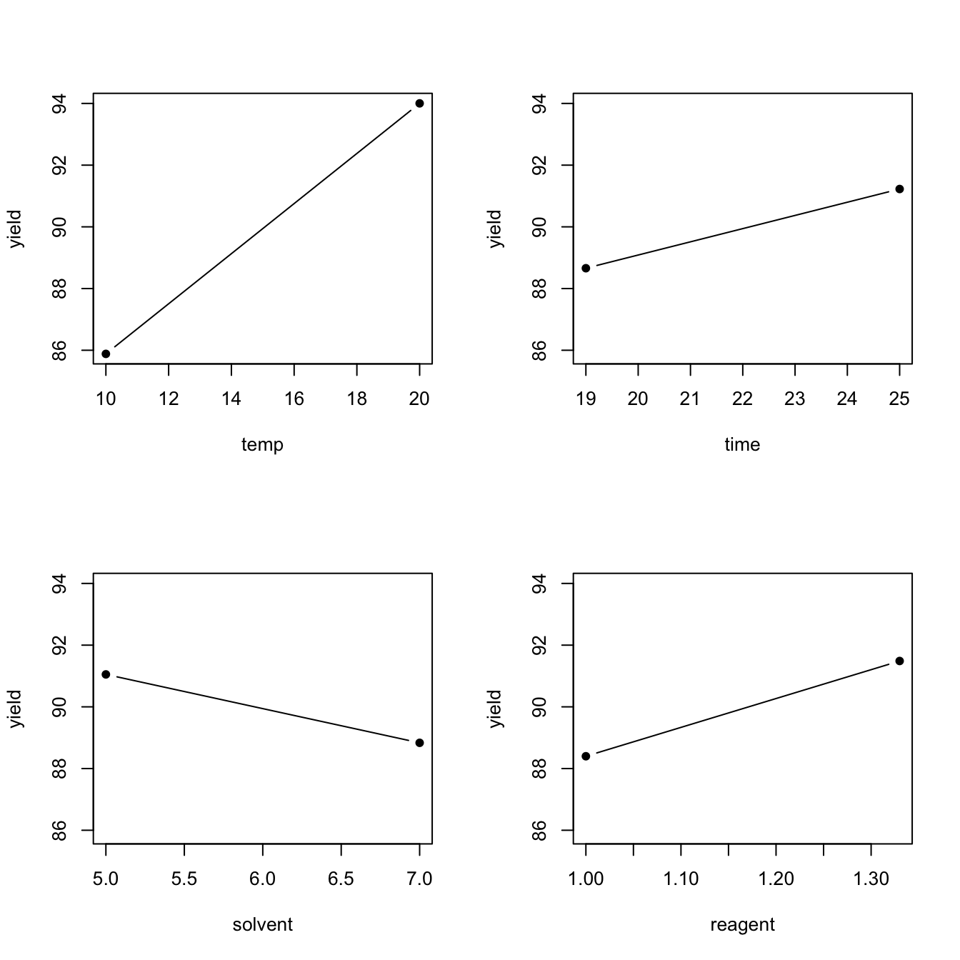
Figure 4.1: Desilylation experiment: main effect plots
4.1.2 Interactions
Another contrast that could be of interest in Example 4.1 has coefficients
\[ \boldsymbol{c}^{\mathrm{T}} = (\boldsymbol{1}_4^{\mathrm{T}}, -\boldsymbol{1}_8^{\mathrm{T}}, \boldsymbol{1}_4^{\mathrm{T}}) / 8 \,, \] where the divisor \(8 = 2^{f-1} = 2^3\).
This contrast measures the difference between the average treatment effect from treatments 1-4, 13-16 and treatments 5-12. Checking back against Table 4.1, we see this is comparing those treatments where solvent and reagent are both set to their low (1-4) or high (13-16) level against those treatments where one of the two factors is set high and the other is set low (5-12).
Focusing on reagent, if the effect of this factor on the response was independent of the level to which solvent has been set, you would expect this contrast to be zero - changing from the high to low level of reagent should affect the response in the same way, regardless of the setting of solvent. This argument can be reversed, focussing on the effect of solvent. Therefore, if this contrast is large, we say the two factors interact.
sol_reg_int.emmc <- function(levels, ...)
  data.frame('reagent x solvent' = .125 * c(rep(1, 4), rep(-1, 8), rep(1, 4)))
emmeans::contrast(desilylation.emm, 'sol_reg_int')
## contrast estimate SE df t.ratio p.value
## reagent.x.solvent 0.49 NaN 0 NaN NaNFor Example 4.1, this interaction contrast seems quite small, although of course without an estimate of the standard error we are still lacking a formal method to judge this.
It is somewhat more informative to consider the above interaction contrast as the average difference in two “sub-contrasts”
\[
\boldsymbol{c}^{\mathrm{T}}\boldsymbol{\tau} = \frac{1}{2}\left\{\frac{1}{4}\left(\tau_{13} + \tau_{14} + \tau_{15} + \tau_{16} - \tau_5 - \tau_6 - \tau_7 - \tau_8\right)
- \frac{1}{4}\left(\tau_9 + \tau_{10} + \tau_{11} + \tau_{12} - \tau_1 - \tau_2 - \tau_3 - \tau_4\right) \right\}\,,
\]
The first component in the above expression is the effect of changing reagent from high to low given solvent is set to it’s high level. The second component the effect of changing reagent from high to low given solvent is set to it’s low level. This leads to our definition of a two-factor interaction.
Definition 4.2 The two-factor interaction between factors \(A\) and \(B\) is defined as the average difference in main effect of factor \(A\) when computed at the high and low levels of factor \(B\).
\[\begin{align*} \mbox{Int}(A, B) & = \frac{1}{2}\left\{\mbox{ME}(A\mid B+) - \mbox{ME}(A \mid B-)\right\} \\ & = \frac{1}{2}\left\{\mbox{ME}(B \mid A+) - \mbox{ME}(B \mid A-)\right\} \\ & = \frac{1}{2}\left\{\bar{y}(A+, B+) - \bar{y}(A-, B+) - \bar{y}(A+, B-) + \bar{y}(A-, B-)\right\}\,, \end{align*}\]
where \(\bar{y}(A+, B-)\) is the average response when factor \(A\) is set to its high level and factor \(B\) is set to its low level, averaged across all combinations of levels of the other factors, and other averages are defined similarly. The conditional main effects of factor \(A\) when factor \(B\) is set to its high level is defined as
\[ \mbox{ME}(A\mid B+) = \bar{y}(A+, B+) - \bar{y}(A-, B+)\,, \]
with similar definitions for other conditional main effects.
As the sum of the squared contrast coefficients is the same for two-factor interactions as for main effects, the variance of the contrast estimator is also the same.
\[ \mbox{var}\left\{\mbox{Int}(A, B)\right\} = \frac{4\sigma^2}{n}\,. \] For Example 4.1 we can calculate two-factor interactions for all \({4 \choose 2} = 6\) pairs of factors. The simplest way to calculate the contrast coefficients is as the elementwise, or Hadamard, product25 of the unscaled main effect contrasts (before dividing by \(2^{f-1}\)).
fac.contrasts.int.emmc <- function(levs, ...) {
  with(sqrt(8) * main_effect_contrasts, {
    data.frame('tem_x_tim' = temp * time,
               'tem_x_sol' = temp * solvent,
               'tem_x_rea' = temp * reagent,
               'tim_x_sol' = time * solvent,
               'tim_x_rea' = time * reagent,
               'sol_x_rea' = solvent * reagent)
  })
}
two_fi_contrasts <- fac.contrasts.int.emmc()
rownames(two_fi_contrasts) <- paste("Trt", 1:16)
knitr::kable(two_fi_contrasts, caption = 'Desilylation experiment: two-factor interaction contrast coefficients')| tem_x_tim | tem_x_sol | tem_x_rea | tim_x_sol | tim_x_rea | sol_x_rea | |
|---|---|---|---|---|---|---|
| Trt 1 | 0.125 | 0.125 | 0.125 | 0.125 | 0.125 | 0.125 |
| Trt 2 | -0.125 | -0.125 | -0.125 | 0.125 | 0.125 | 0.125 |
| Trt 3 | -0.125 | 0.125 | 0.125 | -0.125 | -0.125 | 0.125 |
| Trt 4 | 0.125 | -0.125 | -0.125 | -0.125 | -0.125 | 0.125 |
| Trt 5 | 0.125 | -0.125 | 0.125 | -0.125 | 0.125 | -0.125 |
| Trt 6 | -0.125 | 0.125 | -0.125 | -0.125 | 0.125 | -0.125 |
| Trt 7 | -0.125 | -0.125 | 0.125 | 0.125 | -0.125 | -0.125 |
| Trt 8 | 0.125 | 0.125 | -0.125 | 0.125 | -0.125 | -0.125 |
| Trt 9 | 0.125 | 0.125 | -0.125 | 0.125 | -0.125 | -0.125 |
| Trt 10 | -0.125 | -0.125 | 0.125 | 0.125 | -0.125 | -0.125 |
| Trt 11 | -0.125 | 0.125 | -0.125 | -0.125 | 0.125 | -0.125 |
| Trt 12 | 0.125 | -0.125 | 0.125 | -0.125 | 0.125 | -0.125 |
| Trt 13 | 0.125 | -0.125 | -0.125 | -0.125 | -0.125 | 0.125 |
| Trt 14 | -0.125 | 0.125 | 0.125 | -0.125 | -0.125 | 0.125 |
| Trt 15 | -0.125 | -0.125 | -0.125 | 0.125 | 0.125 | 0.125 |
| Trt 16 | 0.125 | 0.125 | 0.125 | 0.125 | 0.125 | 0.125 |
Estimates of the interaction contrasts can again by found by considering the equivalent contrasts in the observed treatment means.
##             [,1]
## tem_x_tim -2.357
## tem_x_sol  2.358
## tem_x_rea -2.773
## tim_x_sol  0.440
## tim_x_rea -0.645
## sol_x_rea 0.490## contrast estimate SE df t.ratio p.value
## tem_x_tim -2.357 NaN 0 NaN NaN
## tem_x_sol 2.357 NaN 0 NaN NaN
## tem_x_rea -2.772 NaN 0 NaN NaN
## tim_x_sol 0.440 NaN 0 NaN NaN
## tim_x_rea -0.645 NaN 0 NaN NaN
## sol_x_rea 0.490 NaN 0 NaN NaNAs with main effects, interactions are often displayed graphically using interaction plots, plotting average responses for each pairwise combination of factors, joined by lines.
plotmin <- min(desilylation$yield)
plotmax <- max(desilylation$yield)
par(cex = 2)
layout(matrix(c(1, 2, 3, 4, 5, 6), nrow = 3, ncol = 2, byrow = TRUE), respect = T)

with(desilylation, {
  interaction.plot(temp, time, yield, type = "b", pch = 16, legend = F,
                   ylim = c(plotmin, plotmax))
  legend("bottomright", legend = c("Time = 19", "Time = 25"), lty = 2:1, cex = .75)
  interaction.plot(temp, solvent, yield, type = "b", pch = 16, legend = F,
                   ylim = c(plotmin, plotmax))
  legend("bottomright", legend = c("Solvent = 5", "Solvent = 7"), lty = 2:1, cex = .75)
  interaction.plot(temp, reagent, yield, type = "b", pch = 16, legend = F,
                   ylim = c(plotmin, plotmax))
  legend("bottomright", legend = c("Reagent = 1", "Reagent = 1.33"), lty = 2:1, cex = .75)
  interaction.plot(time, solvent, yield, type = "b", pch = 16, legend = F,
                   ylim = c(plotmin, plotmax))
  legend("bottomright", legend = c("Solvent = 5", "Solvent = 7"), lty = 2:1, cex = .75)
  interaction.plot(time, reagent, yield, type = "b", pch = 16, legend = F,
                   ylim = c(plotmin, plotmax))
  legend("bottomright", legend = c("Reagent = 1", "Reagent = 1.33"), lty = 2:1, cex = .75)
  interaction.plot(solvent, reagent, yield, type = "b", pch = 16, legend = F,
                   ylim = c(plotmin, plotmax))
  legend("bottomright", legend = c("Reagent = 1", "Reagent = 1.33"), lty = 2:1, cex = .75)
})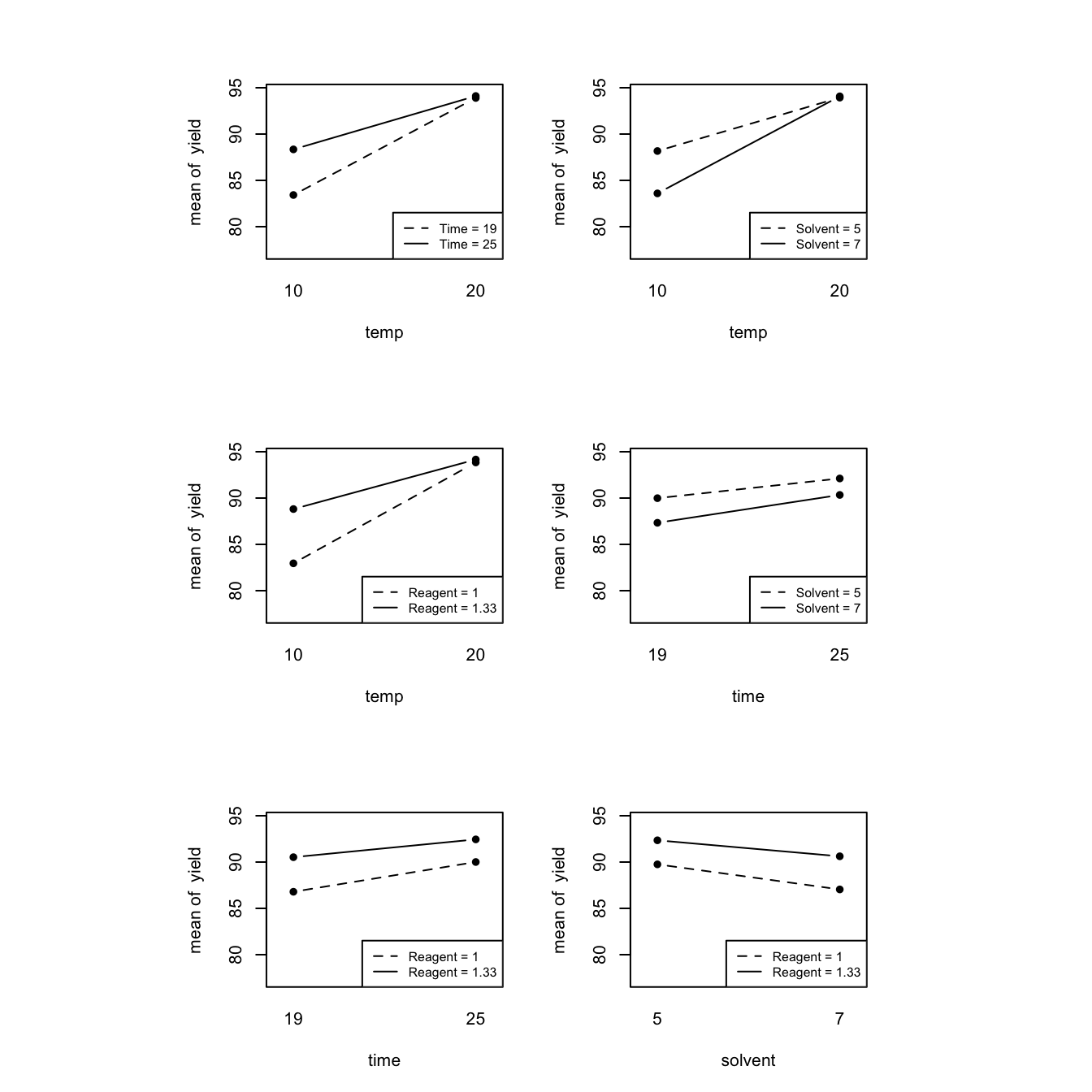
Figure 4.2: Desilylation experiment: two-factor interaction plots
Parallel lines in an interaction plot indicate no (or very small) interaction (time and solvent, time and reagent, solvent and reagent). The three interactions with temp all demonstrate much more robust behaviour at the high level; changing time, solvent or reagent makes little difference to the response at the high level of temp, and much less difference than at the low level of temp.
If a system displays important interactions, the main effects of factors involved in those interactions should no longer be interpreted. For example, it makes little sense to discuss the main effect of temp when is changes so much with the level of reagent (from strongly positive when reagent is low to quite small when reagent is high).
Higher order interactions can be defined similarly, as average differences in lower-order effects. For example, a three-factor interaction measures how a two-factor interaction changes with the levels of a third factor.
\[\begin{align*} \mbox{Int}(A, B, C) & = \frac{1}{2}\left\{\mbox{Int}(A, B \mid C+) - \mbox{Int}(A, B \mid C-)\right\} \\ & = \frac{1}{2}\left\{\mbox{Int}(A, C \mid B+) - \mbox{Int}(A, C \mid B-)\right\} \\ & = \frac{1}{2}\left\{\mbox{Int}(B, C \mid A+) - \mbox{Int}(B, C \mid A-)\right\}\,, \\ \end{align*}\]
where
\[ \mbox{Int}(A, B \mid C+) = \frac{1}{2}\left\{\bar{y}(A+, B+, C+) - \bar{y}(A-, B+, C+) - \bar{y}(A+, B-, C+) + \bar{y}(A-, B-, C+)\right\} \] is the interaction between factors \(A\) and \(B\) using only those treatments where factor \(C\) is set to it’s high level. Higher order interaction contrasts can again be constructed by (multiple) hadamard products of (unscaled) main effect contrasts.
Definition 4.3 A factorial effect is a main effect or interaction contrast defined on a factorial experiment. For a \(2^f\) factorial experiment with \(f\) factors, there are \(2^f-1\) factorial effects, ranging from main effects to the interaction between all \(f\) factors. The contrast coefficients in a factorial contrast all take the form \(c_i = \pm 1 / 2^{f-1}\).
For Example 4.1, we can now calculate all the factorial effects.
## hadamard products
unscaled_me_contrasts <- 8 * main_effect_contrasts
factorial_contrasts <- model.matrix(~.^4, unscaled_me_contrasts)[, -1] / 8

## all factorial effects - directly, as there is no treatment replication
t(factorial_contrasts) %*% yield
## [,1]
## temp 8.1200
## time 2.5675
## solvent -2.2175
## reagent 3.0875
## temp:time -2.3575
## temp:solvent 2.3575
## temp:reagent -2.7725
## time:solvent 0.4400
## time:reagent -0.6450
## solvent:reagent 0.4900
## temp:time:solvent 0.2450
## temp:time:reagent 0.1950
## temp:solvent:reagent -0.0300
## time:solvent:reagent -0.2375
## temp:time:solvent:reagent 0.1925## using emmeans
factorial_contrasts.emmc <- function(levs, ...) data.frame(factorial_contrasts)
desilylation.effs <- emmeans::contrast(desilylation.emm, 'factorial_contrasts')
desilylation.effs## contrast estimate SE df t.ratio p.value
## temp 8.120 NaN 0 NaN NaN
## time 2.567 NaN 0 NaN NaN
## solvent -2.218 NaN 0 NaN NaN
## reagent 3.088 NaN 0 NaN NaN
## temp.time -2.357 NaN 0 NaN NaN
## temp.solvent 2.358 NaN 0 NaN NaN
## temp.reagent -2.773 NaN 0 NaN NaN
## time.solvent 0.440 NaN 0 NaN NaN
## time.reagent -0.645 NaN 0 NaN NaN
## solvent.reagent 0.490 NaN 0 NaN NaN
## temp.time.solvent 0.245 NaN 0 NaN NaN
## temp.time.reagent 0.195 NaN 0 NaN NaN
## temp.solvent.reagent -0.030 NaN 0 NaN NaN
## time.solvent.reagent -0.238 NaN 0 NaN NaN
## temp.time.solvent.reagent 0.192 NaN 0 NaN NaN4.2 Three principles for factorial effects
Empirical study of many experiments (Box and Meyer, 1986; Li et al., 2006) have demonstrated that the following three principles often hold when analysing factorial experiments.
Definition 4.4 Effect hierarchy: lower-order factorial effects are more likely to be important than higher-order effects; factorial effects of the same order are equally likely to be important.
For example, we would anticipate more large main effects from the analysis of a factorial experiment than two-factor interactions.
Definition 4.5 Effect sparsity: the number of large factorial effects is likely to be small, relative to the total number under study.
This is sometimes called the pareto principle.
Definition 4.6 Effect heredity: interactions are more likely to be important if at least one parent factor also has a large main effect.
These three principles will provide us with some useful guidelines when analysing, and eventually constructing, factorial experiments.
4.3 Normal effect plots for unreplicated factorial designs
The lack of an estmate for \(\sigma^2\) means alternatives to formal inference methods (e.g. hypothesis tests) must be found to assess the size of factorial effects. We will discuss a method that essentially treats the identification of large factorial effects as an outlier identification problem.
Let \(\hat{\theta}_j\) be the \(j\)th estimated factorial effect, with \(\hat{\theta}_j = \sum_{i=1}^tc_{ij}\bar{y}_{i.}\) for \(\boldsymbol{c}_j^{\mathrm{T}} = (c_{1j}, \ldots, c_{tj})\) a vector of factorial contrast coefficients (defining a main effect or interaction). Then the estimator follows a normal distribution
\[ \hat{\theta}_j \sim N\left(\theta_j, \frac{4\sigma^2}{n}\right)\,,\qquad j = 1, \ldots, 2^f-1\,, \] for \(\theta_j\) the true, unknown, value of the factorial effect, \(j = 1,\ldots, 2^f\). Further more, for \(j, l = 1, \ldots 2^f-1; \, j\ne l\),
\[\begin{align*} \mbox{cov}(\hat{\theta}_j, \hat{\theta}_l) & = \mbox{cov}\left(\sum_{i=1}^tc_{ij}\bar{y}_{i.}, \sum_{i=1}^tc_{il}\bar{y}_{i.}\right) \\ & = \sum_{i=1}^tc_{ij}c_{il}\mbox{var}(\bar{y}_{i.}) \\ & = \frac{\sigma^2}{r} \sum_{i=1}^tc_{ij}c_{il} \\ & = 0\,, \\ \end{align*}\]
as \(\sum_{i=1}^tc_{ij}c_{il} = 0\) for \(j\ne l\). That is, the factorial contrasts are independent as the contrast coefficient vectors are orthogonal.
Hence, under the null hypothesis \(H_0: \theta_1 = \cdots = \theta_{2^f-1} = 0\) (all factorial effects are zero), the \(\hat{\theta}_j\) form a sample from independent normally distributed random variables from the distribution
\[\begin{equation} \hat{\theta}_j \sim N\left(0, \frac{4\sigma^2}{n}\right)\,,\qquad j = 1, \ldots, 2^f-1\,. \tag{4.3} \end{equation}\]
To assess evidence against \(H_0\), we can plot the ordered estimates of the factorial effects against the ordered quantiles of a standard normal distribution. Under \(H_0\), the points in this plot should lie on a straightline (the slope of the line will depend on the unknown \(\sigma^2\)). We anticipate that the majority of the effects will be small (effect sparsity), and hence any large effects that lie away from the line are unlikely to come from distribution (4.3) and may be significantly different from zero. We have essentially turned the problem into an outlier identification problem.
For Example 4.1, we can easily produce this plot in R. Table 4.4 gives the ordered factorial effects, which are then plotted against standard normal quantiles in Figure 4.3.
effs <- dplyr::arrange(transform(desilylation.effs)[,1:2], dplyr::desc(estimate))
knitr::kable(effs, caption = "Desilylation experiment: sorted estimated factorial effects")
qqnorm(effs[ ,2], ylab = "Factorial effects", main = "") # note that qqnorm/qqline/qqplot don't require sorted data
qqline(effs[ ,2])| contrast | estimate |
|---|---|
| temp | 8.1200 |
| reagent | 3.0875 |
| time | 2.5675 |
| temp.solvent | 2.3575 |
| solvent.reagent | 0.4900 |
| time.solvent | 0.4400 |
| temp.time.solvent | 0.2450 |
| temp.time.reagent | 0.1950 |
| temp.time.solvent.reagent | 0.1925 |
| temp.solvent.reagent | -0.0300 |
| time.solvent.reagent | -0.2375 |
| time.reagent | -0.6450 |
| solvent | -2.2175 |
| temp.time | -2.3575 |
| temp.reagent | -2.7725 |
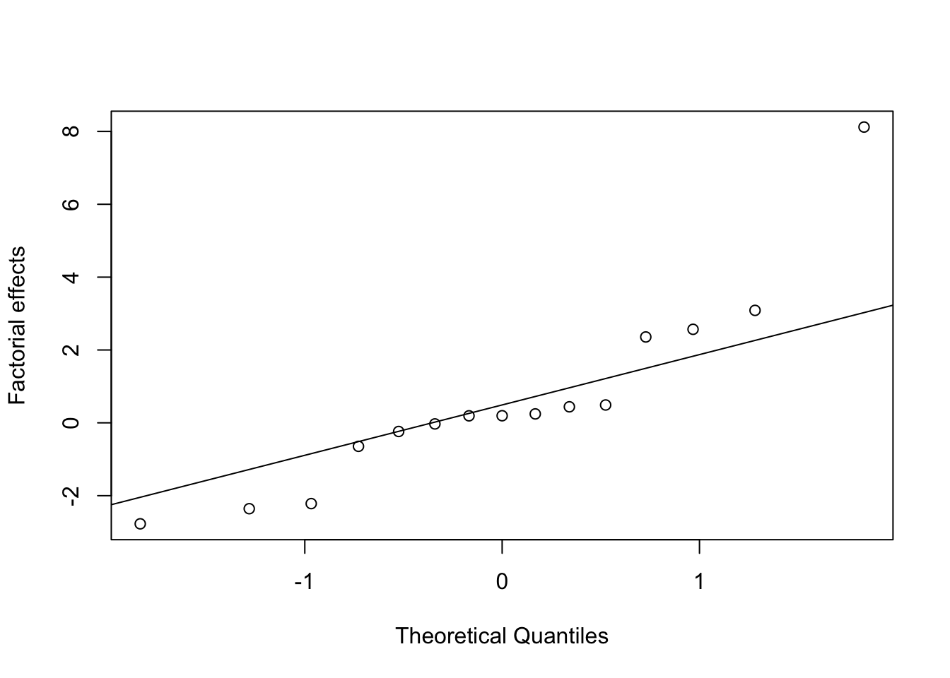
Figure 4.3: Desilylation experiment: normal effects plot
In fact, it is more usual to use a half-normal plot to assess the size of factorial effects, where we plot the sorted absolute values of the estimated effects against the quantiles of a half-normal distribution26
p <- .5 + .5 * (1:16 - .5) /16 # probabilities we will plot against
qqplot(x = qnorm(p), y = abs(effs[,2]), ylab = "Absolute factorial effects",
xlab = "Half-normal quantiles")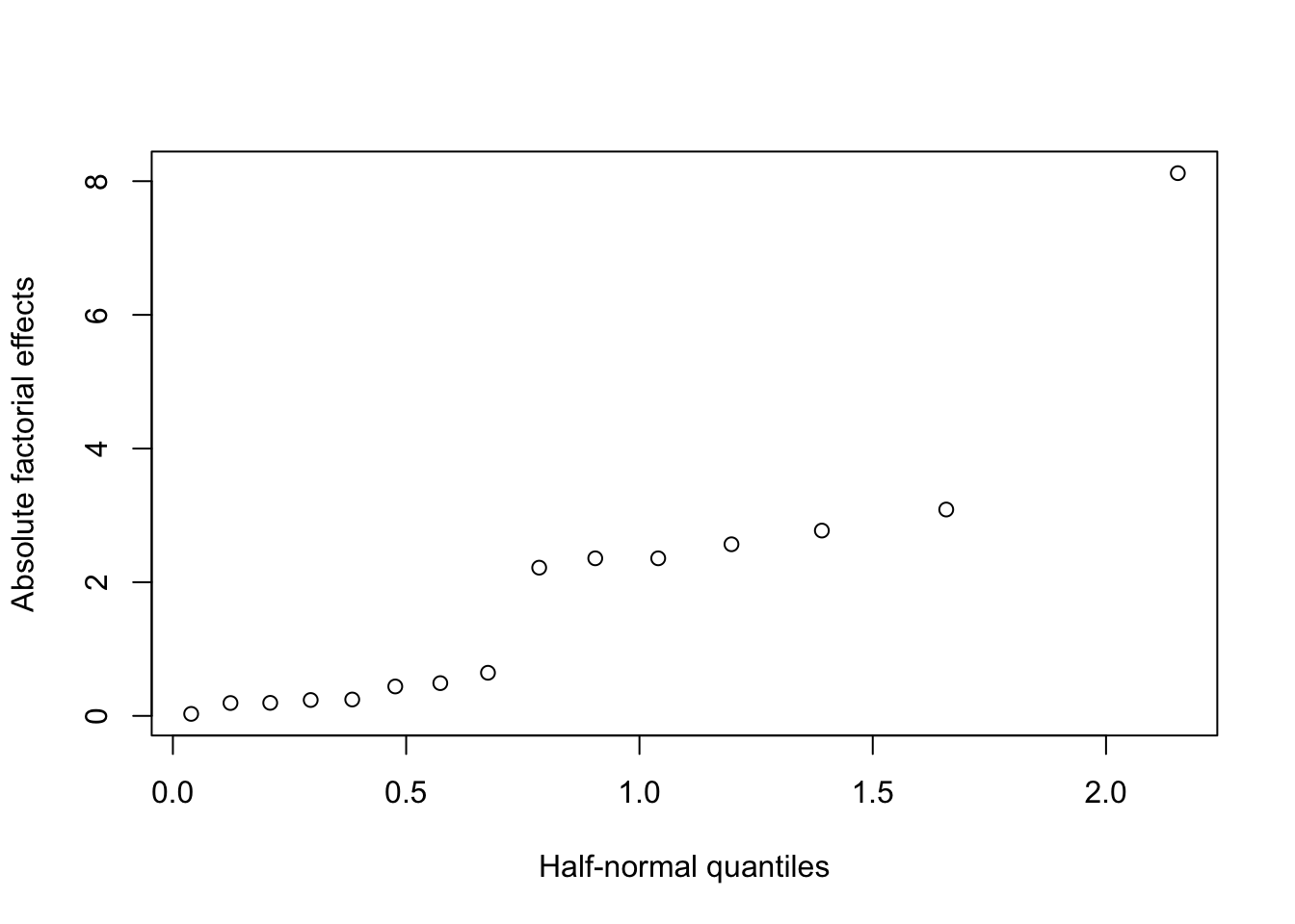
Figure 4.4: Desilylation experiment: half-normal effects plot
The advantage of a half-normal plot such as Figure 4.4 is that we only need to look at effects appearing in the top right corner (significant effects will always appear “above” a hypothetical straight line) and we do not need to worry about comparing large positive and negative values. For these reason, they are usually preferred over normal plots.
For the desilylation experiment, we can see the effects fall into three groups: one effect standing well away from the line, and almost certainly significant (temp, from Table 4.4), then a group of six effects (reagent, time, temp.solvent, solvent, temp.time, temp.reagent) which may be significant, and then a group of 8 much smaller effects.
4.3.1 Lenth’s method for approximate hypothesis testing
The assessment of normal or half-normal effect plots can be quite subjective. Lenth (1989) introduced a simple method for conducting more formal hypothesis testing in unreplicated factorial experiments.
Lenth’s method uses a pseudo standard error (PSE):
\[ \mbox{PSE} = 1.5 \times \mbox{median}_{|\hat{\theta}_i| < 2.5s_0}|\hat{\theta}_i|\,, \] where \(s_0 = 1.5\times \mbox{median} |\hat{\theta}_i|\) is a consistent27 estimator of the standard deviation of the \(\hat{\theta}_i\) under \(H_0: \theta_1 = \cdots=\theta_{2^f-1}=0\). The PSE trims approximately 1%28 of the \(\hat{\theta}_i\) to produce a robust estimator of the standard deviation, in the sense that it is not influenced by large \(\hat{\theta}_i\) belonging to important effects.
For Example 4.1, we can construct the PSE as follows.
s0 <- 1.5 * median(abs(effs[, 2]))
trimmed <- abs(effs[, 2]) < 2.5 * s0
pse <- 1.5 * median(abs(effs[trimmed, 2]))
pse## [1] 0.66The PSE can be used to construct test statistics
\[ t_{\mbox{PSE}, i} = \frac{\hat{\theta}_i}{\mbox{PSE}}\,, \]
which mimic the usual \(t\)-statistics used when an estimate of \(\sigma^2\) is available. These quantities can be compared to reference distribution which was tabulated by Lenth (1989) and simulated in R using the unrepx package.
eff_est <- effs[, 2]
names(eff_est) <- effs[, 1]
lenth_tests <- unrepx::eff.test(eff_est, method = "Lenth")
knitr::kable(lenth_tests, caption = "Desilylation experiment: hypothesis tests using Lenth's method.")| effect | Lenth_PSE | t.ratio | p.value | simult.pval | |
|---|---|---|---|---|---|
| temp | 8.1200 | 0.66 | 12.303 | 0.0001 | 0.0007 |
| reagent | 3.0875 | 0.66 | 4.678 | 0.0037 | 0.0307 |
| temp.reagent | -2.7725 | 0.66 | -4.201 | 0.0054 | 0.0476 |
| time | 2.5675 | 0.66 | 3.890 | 0.0073 | 0.0675 |
| temp.solvent | 2.3575 | 0.66 | 3.572 | 0.0103 | 0.0971 |
| temp.time | -2.3575 | 0.66 | -3.572 | 0.0103 | 0.0971 |
| solvent | -2.2175 | 0.66 | -3.360 | 0.0132 | 0.1200 |
| time.reagent | -0.6450 | 0.66 | -0.977 | 0.3035 | 0.9963 |
| solvent.reagent | 0.4900 | 0.66 | 0.742 | 0.4301 | 1.0000 |
| time.solvent | 0.4400 | 0.66 | 0.667 | 0.5394 | 1.0000 |
| temp.time.solvent | 0.2450 | 0.66 | 0.371 | 0.7335 | 1.0000 |
| time.solvent.reagent | -0.2375 | 0.66 | -0.360 | 0.7406 | 1.0000 |
| temp.time.reagent | 0.1950 | 0.66 | 0.295 | 0.7861 | 1.0000 |
| temp.time.solvent.reagent | 0.1925 | 0.66 | 0.292 | 0.7895 | 1.0000 |
| temp.solvent.reagent | -0.0300 | 0.66 | -0.045 | 0.9667 | 1.0000 |
The function eff.test calculates unadjusted p-values (p.value) and simultaneous p-values (simult.pval) adjusted to account for multiple testing. Using the latter, from Table 4.5 we see that the main effects of temp and reagent are significant at the experiment-wise 5% level and, obeying effect heredity, their interaction (the p-value is borderline, and hovers around 0.05 depending on simulation error).
The package unrepx also provides the function hnplot to display these results graphically by adding a reference line to a half-normal plot; see Figure 4.5. The ME and SME lines indicate the absolute size of effects that would be required to reject \(H_0: \theta_i = 0\) at an individual or experimentwise \(100\alpha\)% level, respectively.
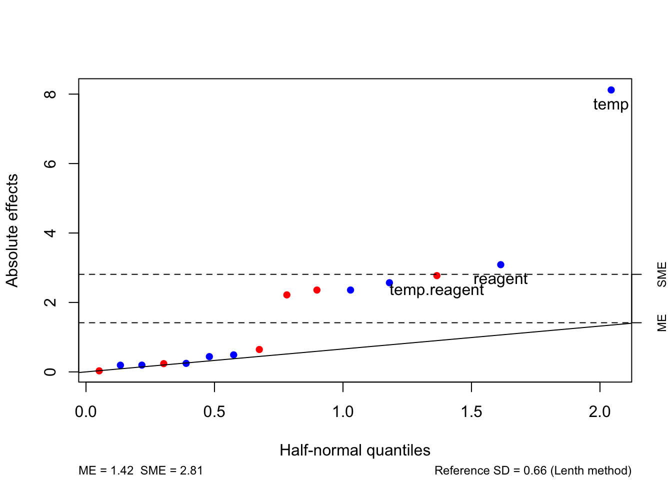
Figure 4.5: Desilylation experiment: half-normal plot with reference lines from Lenth’s method.
Informally, factorial effects with estimates greater than SME are thought highly likely to be significant, and effects between ME and SME are considered somewhat likely to be significant (and still worthy of further investigation if the budget allows).
4.4 Regression modelling for factorial experiments
We have identified \(d = 2^f-1\) factorial effects that we wish to estimate from our experiment. As \(d < t = 2^f\), we can estimate these factorial effects using a full-rank linear regression model.
Let \(t\times d\) matrix \(C\) hold each factorial contrast as a column. Then
\[ \hat{\boldsymbol{\theta}} = C^{\mathrm{T}}\bar{\boldsymbol{y}}\,, \]
with \(\hat{\boldsymbol{\theta}}^{\mathrm{T}} = (\hat{\theta}_1, \ldots, \hat{\theta}_d)\) being the vector of estimated factorial effects and \(\bar{\boldsymbol{y}}^{\mathrm{T}} = (\bar{y}_{1.}, \ldots, \bar{y}_{t.})\) being the vector of treatment means.
We can define an \(n\times d\) expanded contrast matrix as \(\tilde{C} = C \otimes \boldsymbol{1}_r\), where each row of \(\tilde{C}\) gives the contrast coefficients for each run of the experiment. Then,
\[ \hat{\boldsymbol{\theta}} = \frac{1}{r}\tilde{C}^{\mathrm{T}}\boldsymbol{y}\,. \] To illustrate, we will imagine a hypothetical version of Example 4.1 where each treatment was repeated three times (with \(y_{i1} = y_{i2} = y_{i3}\)).
y <- kronecker(desilylation$yield, rep(1, 3)) # hypothetical response vector
C <- factorial_contrasts
Ctilde <- kronecker(C, rep(1, 3))
t(Ctilde) %*% y / 3 # to check## [,1]
## [1,] 8.1200
## [2,] 2.5675
## [3,] -2.2175
## [4,] 3.0875
## [5,] -2.3575
## [6,] 2.3575
## [7,] -2.7725
## [8,] 0.4400
## [9,] -0.6450
## [10,] 0.4900
## [11,] 0.2450
## [12,] 0.1950
## [13,] -0.0300
## [14,] -0.2375
## [15,] 0.1925If we define a model matrix \(X = \frac{2^{f}}{2}\tilde{C}\), then \(X\) is a \(n\times d\) matrix with entries \(\pm 1\) and columns equal to unscaled factorial contrasts. Then
\[\begin{align} \left(X^{\mathrm{T}}X\right)^{-1}X^{\mathrm{T}}\boldsymbol{y}& = \frac{1}{n} \times \frac{2^f}{2}\tilde{C}^{\mathrm{T}}\boldsymbol{y}\tag{4.4}\\ & = \frac{1}{2r}\tilde{C}^{\mathrm{T}}\boldsymbol{y}\\ & = \frac{1}{2}\hat{\boldsymbol{\theta}}\,. \\ \end{align}\]
The left-hand side of equation (4.4) is the least squares estimator \(\hat{\boldsymbol{\beta}}\) from the model
\[ \boldsymbol{y}= \boldsymbol{1}_n\beta_0 + X\boldsymbol{\beta} + \boldsymbol{\varepsilon}\,, \] where \(\boldsymbol{y}\) is the response vector and \(\boldsymbol{\varepsilon}\) the error vector from unit-treatment model (4.1). We have simply re-expressed the mean response as \(\mu + \tau_i = \beta_0 + \boldsymbol{x}_i^{\mathrm{T}}\boldsymbol{\beta}\), where \(d\)-vector \(\boldsymbol{x}_i\) holds the unscaled contrast coefficients for the main effects and interactions.
We can illustrate these connections for Example 4.1.
##                              [,1]
## temp                       8.1200
## time                       2.5675
## solvent                   -2.2175
## reagent                    3.0875
## temp:time                 -2.3575
## temp:solvent               2.3575
## temp:reagent              -2.7725
## time:solvent               0.4400
## time:reagent              -0.6450
## solvent:reagent            0.4900
## temp:time:solvent          0.2450
## temp:time:reagent          0.1950
## temp:solvent:reagent      -0.0300
## time:solvent:reagent      -0.2375
## temp:time:solvent:reagent 0.1925The more usual way to think about this modelling approach is as a regression model with \(f\) (quantitative29) variables, labelled \(x_1, \ldots, x_{2^f-1}\), scaled to lie in the interval \([-1, 1]\) (in fact, they just take values \(\pm 1\)). We can then fit a regression model in these variables, and include products of these variables to represent interactions. We usually also include the intercept term. For Example 4.1:
desilylation.df <- dplyr::mutate(desilylation,
                                      across(.cols = temp:reagent,
                                             ~ as.numeric(as.character(.x))))
desilylation.df <- dplyr::select(desilylation.df, -c(trt))
desilylation.df <- dplyr::mutate(desilylation.df, across(.cols = temp:reagent,
                                               ~ scales::rescale(.x, to = c(-1, 1))))
desilylation_reg.lm <- lm(yield ~ (.) ^ 4, data = desilylation.df)
knitr::kable(2 * coef(desilylation_reg.lm)[-1], caption = "Desilylation example: factorial effects calculated using a regression model.")| x | |
|---|---|
| temp | 8.1200 |
| time | 2.5675 |
| solvent | -2.2175 |
| reagent | 3.0875 |
| temp:time | -2.3575 |
| temp:solvent | 2.3575 |
| temp:reagent | -2.7725 |
| time:solvent | 0.4400 |
| time:reagent | -0.6450 |
| solvent:reagent | 0.4900 |
| temp:time:solvent | 0.2450 |
| temp:time:reagent | 0.1950 |
| temp:solvent:reagent | -0.0300 |
| time:solvent:reagent | -0.2375 |
| temp:time:solvent:reagent | 0.1925 |
A regression modelling approach is usually more straightforward to apply than defining contrasts in the unit-treatment model, and makes clearer the connection between interaction contrasts and products of main effect contrasts (automatically defined in a regression model). It also enables us to make use of the effects package in R to quickly produce main effect and interaction plots.
temp_x_time <- effects::Effect(c("temp", "time"), desilylation_reg.lm, xlevels = list(time = c(-1, 1)), se = F)
plot(temp_x_time, main = "", rug = F, x.var = "temp", ylim = c(80, 100))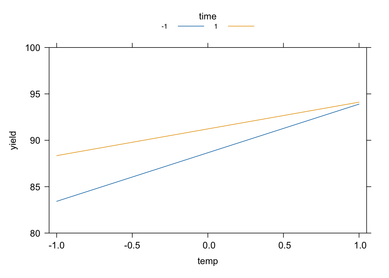
Figure 4.6: Desilylation experiment: interaction plot generated using the effects package.
4.4.1 ANOVA for factorial experiments
The basic ANOVA table has the following form.
| Source | Degress of Freedom | (Sequential) Sum of Squares | Mean Square |
|---|---|---|---|
| Regression | \(2^f-1\) | \(\sum_{j=1}^{2^f-1}n\hat{\beta}_j^2 - n\bar{y}^2\) | Reg SS/\((2^f-1)\) |
| Residual | \(2^f(r-1)\) | \((\boldsymbol{Y}-X\hat{\boldsymbol{\beta}})^{\textrm{T}}(\boldsymbol{Y}-X\hat{\boldsymbol{\beta}})\) | RSS/\((2^f(r-1))\) |
| Total | \(2^fr-1\) | \(\boldsymbol{Y}^{\textrm{T}}\boldsymbol{Y}-n\bar{Y}^{2}\) |
The regression sum of squares for a factorial experiment has a very simple form. If we include an intercept column in \(X\), from Section 1.5.1,
\[\begin{align*} \mbox{Regression SS} & = \mbox{RSS(null)} - \mbox{RSS} \\ & = \hat{\boldsymbol{\beta}}^{\mathrm{T}}X^{\mathrm{T}}X\hat{\boldsymbol{\beta}} - n\bar{y}^2 \\ & = \sum_{j=1}^{2^f-1}n\hat{\beta}_j^2 - n\bar{y}^2\,, \end{align*}\]
as \(X^{\mathrm{T}}X = nI_{2^f}\). Hence, the \(j\)th factorial effect contributes \(n\hat{\beta}_j^2\) to the regression sum if squares, and this quantity can be used to construct a test statistic if \(r>1\) and hence an estimate of \(\sigma^2\) is available. For Example 4.1, the regression sum of squares and ANOVA table are given in Tables 4.8 and 4.9.
ss <- nrow(desilylation) * coef(desilylation_reg.lm)^2
regss <- sum(ss) - nrow(desilylation) * mean(desilylation$yield)^2
names(regss) <- "Regression"
knitr::kable(c(regss, ss[-1]), col.names = "Sum Sq.", caption = "Desilylation experiment: regression sums of squares for each factorial effect calculated directly.")| Sum Sq. | |
|---|---|
| Regression | 427.2837 |
| temp | 263.7376 |
| time | 26.3682 |
| solvent | 19.6692 |
| reagent | 38.1306 |
| temp:time | 22.2312 |
| temp:solvent | 22.2312 |
| temp:reagent | 30.7470 |
| time:solvent | 0.7744 |
| time:reagent | 1.6641 |
| solvent:reagent | 0.9604 |
| temp:time:solvent | 0.2401 |
| temp:time:reagent | 0.1521 |
| temp:solvent:reagent | 0.0036 |
| time:solvent:reagent | 0.2256 |
| temp:time:solvent:reagent | 0.1482 |
knitr::kable(anova(desilylation_reg.lm)[, 1:2], caption = "Desilylation experiment: ANOVA table from `anova` function.")## Warning in anova.lm(desilylation_reg.lm): ANOVA F-tests on an essentially
## perfect fit are unreliable| Df | Sum Sq | |
|---|---|---|
| temp | 1 | 263.7376 |
| time | 1 | 26.3682 |
| solvent | 1 | 19.6692 |
| reagent | 1 | 38.1306 |
| temp:time | 1 | 22.2312 |
| temp:solvent | 1 | 22.2312 |
| temp:reagent | 1 | 30.7470 |
| time:solvent | 1 | 0.7744 |
| time:reagent | 1 | 1.6641 |
| solvent:reagent | 1 | 0.9604 |
| temp:time:solvent | 1 | 0.2401 |
| temp:time:reagent | 1 | 0.1521 |
| temp:solvent:reagent | 1 | 0.0036 |
| time:solvent:reagent | 1 | 0.2256 |
| temp:time:solvent:reagent | 1 | 0.1482 |
| Residuals | 0 | 0.0000 |
4.5 Exercises
A reactor experiment that was presented by Box, Hunter and Hunter (2005, pp259-261) that used a full factorial design for \(m=5\) factors, each at two levels, to investigate the effect of feed rate (litres/min), catalyst (%), agitation rate (rpm), temperature (C) and concentration (%) on the percentage reacted. The levels of the experimental factors will be coded as \(-1\) for low level, and \(1\) for high level. Table 4.10 presents the true factor settings corresponding to these coded values.
Table 4.10: Factor levels for the full factorial reactor experiment Factor Low level (\(-1\)) High level (\(1\)) Feed Rate (litres/min) 10 15 Catalyst (%) 1 2 Agitation Rate (rpm) 100 120 Temperature (C) 140 180 Concentration (%) 3 6 The data from this experiment is given in Table 4.11.
reactor.frf2 <- FrF2::FrF2(nruns = 32, nfactors = 5, randomize = F,
                           factor.names = c("FR", "Cat", "AR", "Temp", "Conc"))
y <- c(61, 53, 63, 61, 53, 56, 54, 61, 69, 61, 94, 93, 66, 60, 95, 98, 56, 63,
       70, 65, 59, 55, 67, 65, 44, 45, 78, 77, 49, 42, 81, 82)
reactor <- data.frame(reactor.frf2, pre.react = y)
knitr::kable(reactor, caption = "Reactor experiment.")
Table 4.11: Reactor experiment. FR Cat AR Temp Conc pre.react -1 -1 -1 -1 -1 61 1 -1 -1 -1 -1 53 -1 1 -1 -1 -1 63 1 1 -1 -1 -1 61 -1 -1 1 -1 -1 53 1 -1 1 -1 -1 56 -1 1 1 -1 -1 54 1 1 1 -1 -1 61 -1 -1 -1 1 -1 69 1 -1 -1 1 -1 61 -1 1 -1 1 -1 94 1 1 -1 1 -1 93 -1 -1 1 1 -1 66 1 -1 1 1 -1 60 -1 1 1 1 -1 95 1 1 1 1 -1 98 -1 -1 -1 -1 1 56 1 -1 -1 -1 1 63 -1 1 -1 -1 1 70 1 1 -1 -1 1 65 -1 -1 1 -1 1 59 1 -1 1 -1 1 55 -1 1 1 -1 1 67 1 1 1 -1 1 65 -1 -1 -1 1 1 44 1 -1 -1 1 1 45 -1 1 -1 1 1 78 1 1 -1 1 1 77 -1 -1 1 1 1 49 1 -1 1 1 1 42 -1 1 1 1 1 81 1 1 1 1 1 82 Estimate all the factorial effects from this experiment, and use a half-normal plot and Lenth’s method to decide which are significantly different from zero.
Use the
effectspackage to produce main effect and/or interaction plots for each significant factorial effect from part a.Now fit a regression model that only includes terms corresponding to main effects and two-factor interactions. How many degrees of freedom does this model use? What does this mean for the estimation of \(\sigma^2\)? How does the estimate of \(\sigma^2\) from this model relate to your analysis in part a?
Solution
- We will estimate the factorial effects as twice the corresponding regression parameters.
reactor <- dplyr::mutate(reactor, across(.cols = FR:Conc,
                                         ~ as.numeric(as.character(.x))))
reactor.lm <- lm(pre.react ~ (.) ^ 5, data = reactor)
fac.effects <- 2 * coef(reactor.lm)[-1]
knitr::kable(fac.effects, caption = "Reactor experiment: estimated factorial effects.")| x | |
|---|---|
| FR | -1.375 |
| Cat | 19.500 |
| AR | -0.625 |
| Temp | 10.750 |
| Conc | -6.250 |
| FR:Cat | 1.375 |
| FR:AR | 0.750 |
| FR:Temp | -0.875 |
| FR:Conc | 0.125 |
| Cat:AR | 0.875 |
| Cat:Temp | 13.250 |
| Cat:Conc | 2.000 |
| AR:Temp | 2.125 |
| AR:Conc | 0.875 |
| Temp:Conc | -11.000 |
| FR:Cat:AR | 1.500 |
| FR:Cat:Temp | 1.375 |
| FR:Cat:Conc | -1.875 |
| FR:AR:Temp | -0.750 |
| FR:AR:Conc | -2.500 |
| FR:Temp:Conc | 0.625 |
| Cat:AR:Temp | 1.125 |
| Cat:AR:Conc | 0.125 |
| Cat:Temp:Conc | -0.250 |
| AR:Temp:Conc | 0.125 |
| FR:Cat:AR:Temp | 0.000 |
| FR:Cat:AR:Conc | 1.500 |
| FR:Cat:Temp:Conc | 0.625 |
| FR:AR:Temp:Conc | 1.000 |
| Cat:AR:Temp:Conc | -0.625 |
| FR:Cat:AR:Temp:Conc | -0.500 |
There are several large factorial effects, including the main effects of Catalyst and Temperature and the interaction between these factors, and the interaction between Concentration and Temperature. We can assess their significance using a half-normal plot and Lenth’s method.
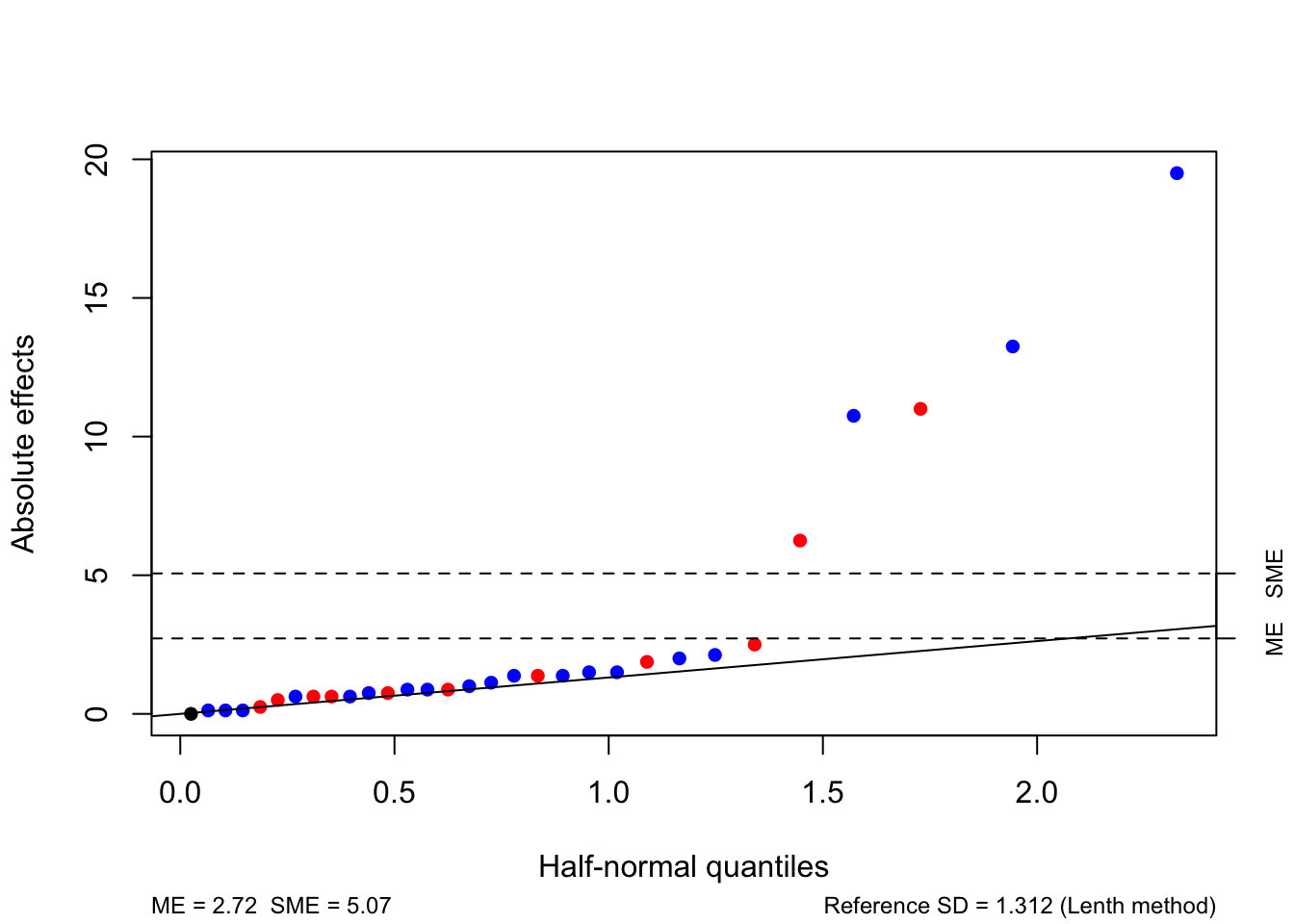
We see that PSE = 1.3125, giving individual and simultaneous margins of error of 2.7484 and 5.195, respectively (where the latter is adjusted for multiple testing). There is a very clear distinction between the five effects which are largest in absolute value and the other factorial effects, which form a very clear line. The five of the largest effects are given in Table 4.13, are all greater than both margins of error and can be declared as significant.
knitr::kable(fac.effects[abs(fac.effects) > unrepx::ME(fac.effects,
                                                       method = "Lenth")[2]],
caption = "Reactor experiment: factorial effects significantly different from zero via Lenth's method.")| x | |
|---|---|
| Cat | 19.50 |
| Temp | 10.75 |
| Conc | -6.25 |
| Cat:Temp | 13.25 |
| Temp:Conc | -11.00 |
- We will produce plots for the interactions between Catalyst and Temperature and Temperature and Concentration. We will not produce main effect plots for Catalyst and Temperature, as these are involved in the large interactions.
Cat_x_Temp <- effects::Effect(c("Cat", "Temp"), reactor.lm,
                              xlevels = list(Cat = c(-1, 1), Temp = c(-1, 1)),
                              se = F)
Temp_x_Conc <- effects::Effect(c("Temp", "Conc"), reactor.lm,
                               xlevels = list(Conc = c(-1, 1), Temp = c(-1, 1)),
                               se = F)
plot(Cat_x_Temp, style = "stacked", main = "", rug = F, x.var = "Cat",
     ylim = c(50, 90))
plot(Temp_x_Conc, style = "stacked", main = "", rug = F, x.var = "Conc",
     ylim = c(50, 90))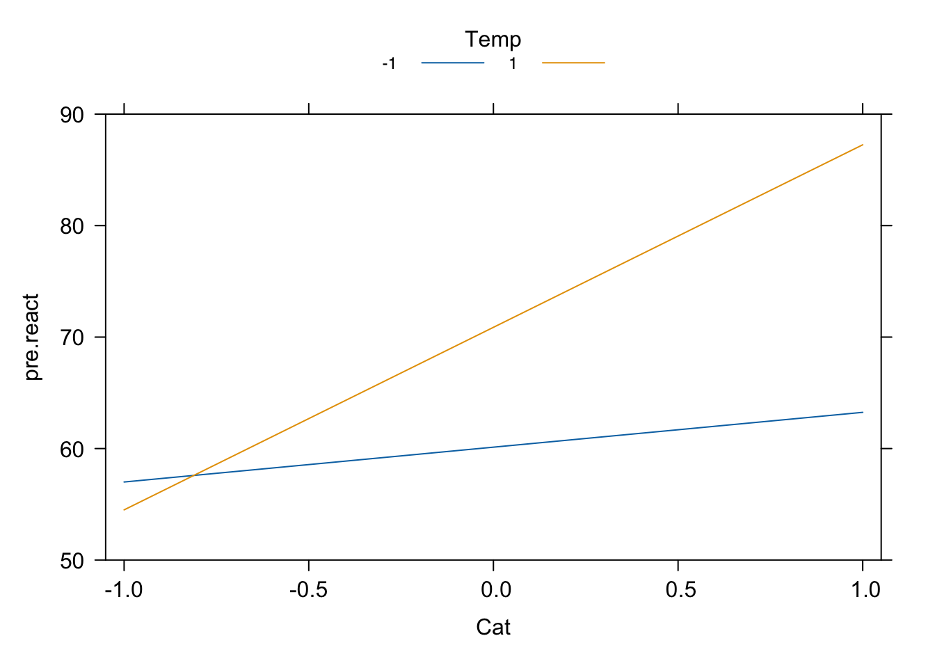
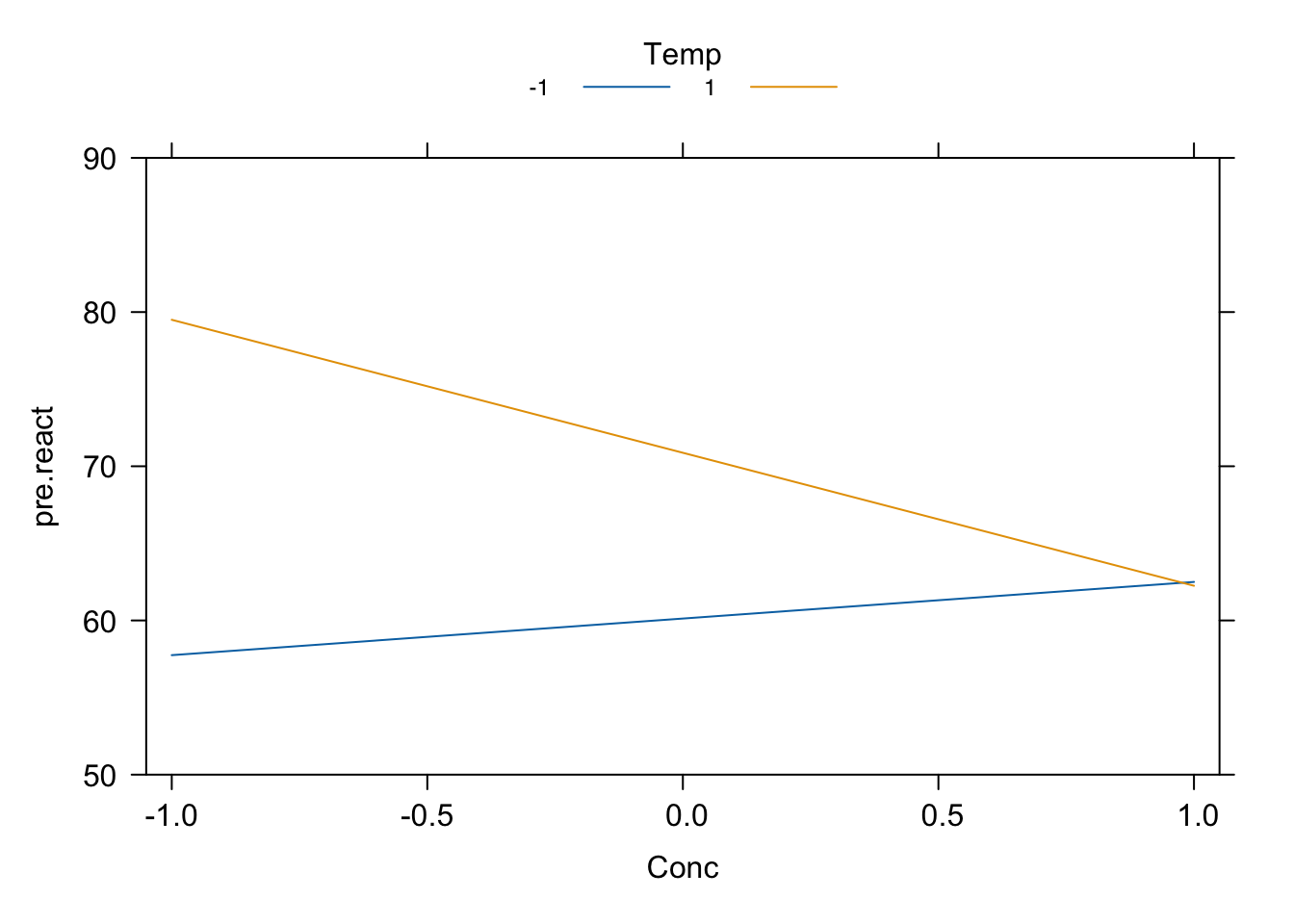
Figure 4.7: Reactor experiment: interaction plots.
Notice that changing the level of Temperature changes substantial the effect of both Catalyst and Concentration on the response; in particular, the effect of Concentration changes sign depending on the level of Temperature.
- We start by fiting the reduced regression model.
##
## Call:
## lm(formula = pre.react ~ (.)^2, data = reactor)
##
## Residuals:
##    Min     1Q Median     3Q    Max
##  -5.00  -1.62  -0.25   1.75   4.50
##
## Coefficients:
##             Estimate Std. Error t value        Pr(>|t|)
## (Intercept)  65.5000     0.5660  115.73         < 2e-16 ***
## FR           -0.6875     0.5660   -1.21           0.242
## Cat           9.7500     0.5660   17.23 0.0000000000094 ***
## AR           -0.3125     0.5660   -0.55           0.588
## Temp          5.3750     0.5660    9.50 0.0000000560392 ***
## Conc         -3.1250     0.5660   -5.52 0.0000464538196 ***
## FR:Cat        0.6875     0.5660    1.21           0.242
## FR:AR         0.3750     0.5660    0.66           0.517
## FR:Temp      -0.4375     0.5660   -0.77           0.451
## FR:Conc       0.0625     0.5660    0.11           0.913
## Cat:AR        0.4375     0.5660    0.77           0.451
## Cat:Temp      6.6250     0.5660   11.71 0.0000000029456 ***
## Cat:Conc      1.0000     0.5660    1.77           0.096 .
## AR:Temp       1.0625     0.5660    1.88           0.079 .
## AR:Conc       0.4375     0.5660    0.77           0.451
## Temp:Conc    -5.5000     0.5660   -9.72 0.0000000408373 ***
## ---
## Signif. codes:  0 '***' 0.001 '**' 0.01 '*' 0.05 '.' 0.1 ' ' 1
##
## Residual standard error: 3.2 on 16 degrees of freedom
## Multiple R-squared:  0.976,  Adjusted R-squared:  0.954
## F-statistic: 44.1 on 15 and 16 DF,  p-value: 0.000000000376
This model includes regression parameters corresponding to \(5 + {5 \choose 2} = 15\) factorial effects, plus the intercept, and hence uses 16 degrees of freedom. The remaining 16 degrees of freedom, which were previously used to estimate three-factor and higher interactions, is now used to estimate \(\sigma^2\), the background variation.
The residual mean square in the reduced model, used to estimate \(\sigma^2\), is the sum of the sums of squares for the higher-order interactions in the original model, divided by 16 (the remaining degrees of freedom).
## [1] 10.25## [1] 10.25(Adapted from Morris, 2011) Consider an unreplicated (\(r=1\)) \(2^6\) factorial experiment. The total sums of squares,
\[ \mbox{Total SS} = \sum_{i=1}^n(y_i - \bar{y})^2\,, \]
has value 2856. Using Lenth’s method, an informal analysis of the data suggests that there are only three important factorial effects, with least squares estimates
- main effect of factor \(A\) = 3
- interaction between factors \(A\) and \(B\) = 4
- interaction between factors \(A\), \(B\) and \(C\) = 2.
If a linear model including only an intercept and these three effects is fitted to the data, what is the value of the residual sum of squares?
Solution
The residual sum of squares has the form
\[ \mbox{RSS} = (\boldsymbol{y}- X\hat {\boldsymbol{\beta}})^{\mathrm{T}}(\boldsymbol{y}- X\hat {\boldsymbol{\beta}})\,, \]
where in this case \(X\) is a \(2^6\times 4\) model matrix, with columsn corresponding to the intercept, main effect of factor \(A\), the interaction between factors \(A\) and \(B\), the interaction between factors \(A\), \(B\) and \(C\). We can rewrite the RSS as
\[\begin{equation*} \begin{split} \mbox{RSS} & = (\boldsymbol{y}- X\hat {\boldsymbol{\beta}})^{\mathrm{T}}(\boldsymbol{y}- X\hat {\boldsymbol{\beta}}) \\ & = \boldsymbol{y}^{\mathrm{T}}\boldsymbol{y}- 2\boldsymbol{y}^{\mathrm{T}}X\hat {\boldsymbol{\beta}} + \hat {\boldsymbol{\beta}}^{\mathrm{T}}X^{\mathrm{T}}X\hat {\boldsymbol{\beta}} \\ & = \boldsymbol{y}^{\mathrm{T}}\boldsymbol{y}- 2\hat {\boldsymbol{\beta}}^{\mathrm{T}}X^{\mathrm{T}}X\hat {\boldsymbol{\beta}} + \hat {\boldsymbol{\beta}}^{\mathrm{T}}X^{\mathrm{T}}X\hat {\boldsymbol{\beta}} \\ & = \boldsymbol{y}^{\mathrm{T}}\boldsymbol{y}- \hat {\boldsymbol{\beta}}^{\mathrm{T}}X^{\mathrm{T}}X\hat {\boldsymbol{\beta}}\,, \end{split} \end{equation*}\]
as \(\boldsymbol{y}^{\mathrm{T}}X = \hat{\boldsymbol{\beta}}^{\mathrm{T}}X^{\mathrm{T}}X\).
Due the matrix \(X\) having orthogonal columns, \(X^{\mathrm{T}}X = 2^fI_{p+1}\), for a model containing coefficients corresponding to \(p\) factorial effects; here, \(p=3\). Hence,
\[ \mbox{RSS} = \boldsymbol{y}^{\mathrm{T}}\boldsymbol{y}- 2^f \sum_{i=0}^{p}\hat{\beta}_i^2\,. \]
Finally, the estimate of the intercept takes the form \(\hat{\beta}_0 = \bar{Y}\), and so
\[\begin{equation*} \begin{split} \mbox{RSS} & = \boldsymbol{y}^{\mathrm{T}}\boldsymbol{y}- 2^f\bar{y}^2 - 2^f\sum_{i=1}^{p}\hat{\beta}_i^2 \\ & = \sum_{i=1}^{2^f}(y_i - \bar{y})^2 - 2^f\sum_{i=1}^{p}\hat{\beta}_i^2 \\ & = \mbox{Total SS} - 2^f\sum_{i=1}^{p}\hat{\beta}_i^2\, \end{split} \end{equation*}\]
Recalling that each regression coefficient is one-half of the corresponding factorial effect, for this example we have:
\[ \mbox{RSS} = 2856 - 2^6(1.5^2 + 2^2 + 1^2) = 2392\,. \]
(Adapted from Morris, 2011) Consider a \(2^7\) experiment with each treatment applied to two units (\(r=2\)). Assume a linear regression model will be fitted containing terms corresponding to all factorial effects.
What is the variance of the estimator of each factorial effect, up to a constant factor \(\sigma^2\)?
What is the variance of the least squares estimator of \(E(y_{11})\), the expected value of an observation with the first treatment applied? You can assume the treatments are given in standard order, so the first treatment is defined by setting all factors to their low level. [The answer is, obviously, the same for \(E(y_{12})\)]. In a practical experimental setting, why is this not a useful quantity to estimate?
What is the variance of the least squares estimator of \(E(y_{11}) - E(y_{21})\)? You may assume that the second treatment has all factors set to their low levels except for the seventh factor.
Solutions
Each factorial contrast is scaled so the variance for the estimator is equal to \(4\sigma^2/n = \sigma^2 / 64\).
\(E(y_{11}) = \boldsymbol{x}_1^{\mathrm{T}}\boldsymbol{\beta}\), where \(\boldsymbol{x}_1^{\mathrm{T}}\) is the row of the \(X\) matrix corresponding to the first treatment and \(\boldsymbol{\beta}\) are the regression coefficients. The estimator is given by
\[ \hat{E}(y_{11}) = \boldsymbol{x}_1^{\mathrm{T}}\hat{\boldsymbol{\beta}}\,, \]
with variance
\[\begin{align*} \mathrm{var}\left\{\hat{E}(y_{11})\right\} & = \mathrm{var}\left\{\boldsymbol{x}_1^{\mathrm{T}}\hat{\boldsymbol{\beta}}\right\} \\ & = \boldsymbol{x}_1^{\mathrm{T}}\mbox{var}(\hat{\boldsymbol{\beta}})\boldsymbol{x}_1 \\ & = \boldsymbol{x}_1^{\mathrm{T}}\left(X^\mathrm{T}X\right)^{-1}\boldsymbol{x}_1\sigma^2 \\ & = \frac{\boldsymbol{x}_1^{\mathrm{T}}\boldsymbol{x}_1\sigma^2}{2^8} \\ & = \frac{2^7\sigma^2}{2^8} \\ & = \sigma^2 / 2\,. \end{align*}\]
This holds for the expected response from any treatment, as \(\boldsymbol{x}_j^{\mathrm{T}}\boldsymbol{x}_j = 2^7\) for all treatments, as each entry of \(\boldsymbol{x}_j\) is equal to \(\pm 1\).
This would not be a useful quantity to estimate in a practical experiment, as it is not a contrast in the treatments. In particular, it depends on the estimate of the overall mean, \(\mu\) or \(\beta_0\) (in the unit-treatment or regression model) that will vary from experiment to experiment.
The expected values of \(y_{11}\) and \(y_{21}\) will only differ in terms involving the seventh factor, which is equal to its low level (-1) for the first treatment and its high level (+1) for the second treatment; all the other terms will cancel. Hence
\[ E(y_{11}) - E(y_{21}) = -2\left(\beta_7 + \sum_{j=1}^6\beta_{j7} + \sum_{j=1}^6\sum_{k=j+1}^6\beta_{jk7} + \ldots + \beta_{1234567}\right)\,. \]
The variance of the estimator has the form
\[\begin{align*} \mathrm{var}\left\{\widehat{E(y_{11}) - E(y_{21})}\right\} & = 4\times\mathrm{var}\bigg(\hat{\beta}_7 + \sum_{j=1}^6\hat{\beta}_{j7} + \sum_{j=1}^6\sum_{k=j+1}^6\hat{\beta}_{jk7} + \\ & \ldots + \hat{\beta}_{1234567}\bigg) \\ & = \frac{4\sigma^2}{2\times 2^7}\sum_{j=0}^6{6 \choose j} \\ & = \frac{\sigma^2}{2^6}\times 64 \\ & = \sigma^2\,. \end{align*}\]
Or, as this is a treatment comparison in a CRD, we have
\[ \hat{E}(y_{11}) - \hat{E}(y_{21}) = \widehat{\boldsymbol{c}^{\mathrm{T}}\boldsymbol{\tau}}\,, \]
where \(\boldsymbol{c}\) corresponds to a pairwise treatment comparison, and hence has one entry equal to +1 and one entry equal to -1. From Section 2.5,
\[\begin{align*} \mathrm{var}\left(\widehat{\boldsymbol{c}^{\mathrm{T}}\boldsymbol{\tau}}\right) & = \sum_{i=1}^tc_i^2\mathrm{var}(\bar{y}_{i.}) \\ & = \sigma^2\sum_{i=1}^tc_i^2/n_i\,, \end{align*}\]
where in this example \(n_i = 2\) for all \(i\) and \(\sum_{i=1}^tc_i^2 = 2\). Hence, the variance is again equal to \(\sigma^2\).
References
Desilylation is a process of removing silyl, SiH\(_3\) a silicon hydride, from a compound.↩︎
For two matrices \(A\) and \(B\) of the same dimension \(m\times n\), the Hadamard product \(A\odot B\) is a matrix of the same dimension with elements given by the elementwise product, \((A\odot B)_{ij} = A_{ij}B_{ij}\).↩︎
The absolute value of a normally distributed random variable follows a half-normal distribution.↩︎
Essentially, \(s_0\) tends in probability to \(\sigma\) as the number of factorial effects tends to infinity.↩︎
Under \(H_0\), the \(\hat{\theta}_i\) come from a mean-zero normal distribution, and about 1% of deviates fall outside \(\pm 2.57\sigma^2\).↩︎
When qualitative factors only have two levels, each regression term only has 1 degree of freedom, and so there is practically little difference from a quantitative variable.↩︎